Most of my professional experience so far has been focused on language and 2D vision. But lately, I’ve been getting very curious about spatial intelligence - the capability to perceive, reason about, and generate in 3D space, not just flat pixels and tokens. If you’ve been following the news, you’ll notice a surge of interest in world models (Yann LeCun’s AMI Labs, Fei-Fei Li’s World Labs) and embodied agents - systems that don’t just process text, but understand and act in physical space. Spatial intelligence is highly relevant here, although it’s more directly related to embodied agents (which need spatial intelligence directly since they have to navigate and act in physical 3D space) than world models (they are about learning an internal model of how the world works - spatial understanding is important for this, but world models also cover physics, causality, and dynamics, not just 3D geometry). This series is my first step into understanding more about spatial intelligence, starting with NeRF.

NeRF: Representing Scenes as Neural Radiance Fields for View Synthesis (Mildenhall et al., 2020) asks: given a set of 2D photos of a scene taken from known camera positions, can we render the scene from any new viewpoint?

NeRF enables AI systems to understand, reconstruct, and navigate 3D environments, by taking sparse 2D images and using a neural network to learn the 3D geometry and appearance of a scene. By transforming 2D inputs into a coherent 3D world representation, NeRF allows AI agents to “see” and navigate physical environments.

First, I recommend that you watch this demo video from the first author of NeRF himself, and prepare to be AMAZED at how crazy good this technology is, although it’s been 6 years since it came out:

The GitHub repo for my PyTorch implementation of mini-NeRF can be found here: halannhile/mini-nerf.

Section 1: Theory

What problem are we solving?
The NeRF representation
Volume rendering
Optimizing a Neural Radiance Field
- 4.1 Positional encoding
- 4.2 Hierarchical volume sampling
Training

Section 2: Code

Overview
Ray generation
Positional encoding
The NeRF network
Volume rendering in code
Hierarchical sampling
Training loop
MPS optimizations

Section 3: Results

Section 4: Recap & what’s next

Useful Resources

Citation

Section 1: Theory

1. What problem are we solving?

Given a set of 2D images with known camera poses, we want to render the scene from new viewpoints. This is called novel view synthesis.

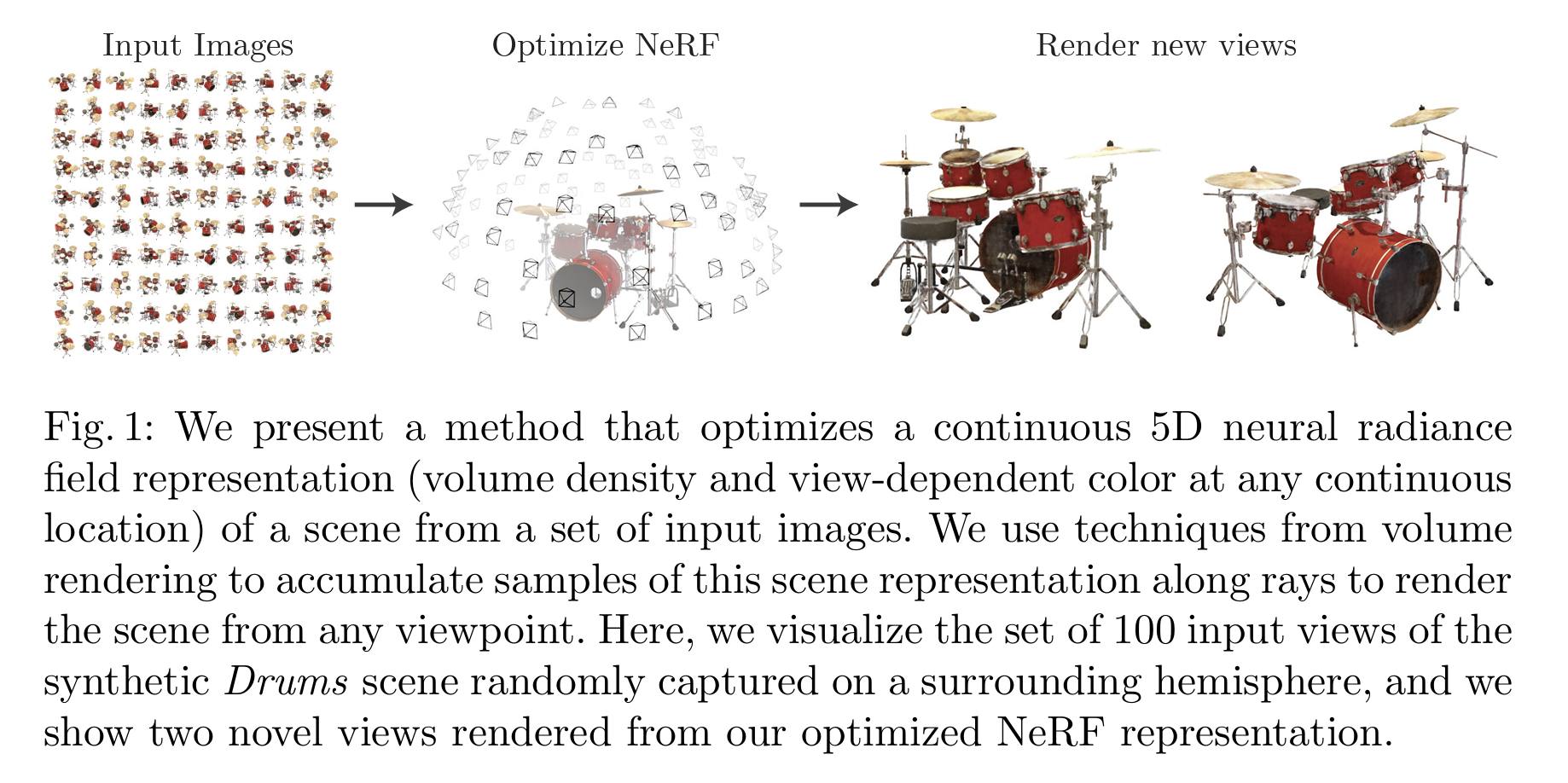
NeRF represents the scene as a neural network and uses differentiable volume rendering to supervise it from 2D pixels only.

2. The NeRF representation

NeRF represents a scene as a continuous function:

$$F_\theta : (\mathbf{x}, \mathbf{d}) \to (\mathbf{c}, \sigma)$$

where:

$\mathbf{x} = (x, y, z)$ is a 3D point in space
$\mathbf{d} = (\theta, \phi)$ is the viewing direction
$\mathbf{c} = (r, g, b)$ is emitted color
$\sigma$ is volume density (opacity)

$F_\theta$ is an MLP. Density $\sigma$ depends only on position. Color $\mathbf{c}$ depends on both position and direction, which lets the model capture view-dependent effects.

3. Volume rendering

This section is a little math-heavy but I want to include all the necessary details here in case you find them useful like I did.

To render a pixel, NeRF shoots a ray from the camera and integrates color along it.

The ray is $\mathbf{r}(t) = \mathbf{o} + t\mathbf{d}$ where $t$ is distance from the camera. The rendered color is:

$$C(\mathbf{r}) = \int_{t_n}^{t_f} T(t), \sigma(\mathbf{r}(t)), \mathbf{c}(\mathbf{r}(t), \mathbf{d}), dt$$

The integrand is $T(t)$ (“ray got here”) × $\sigma(\mathbf{r}(t))$ (“something is here”) × $\mathbf{c}(\mathbf{r}(t), \mathbf{d})$ (“color here”).

$\sigma(\mathbf{r}(t))$ and $\mathbf{c}(\mathbf{r}(t), \mathbf{d})$ make sense, if you refer back to section 2 above on NeRF representation, but where does $T(t)$ come from?

$T(t)$ is transmittance - the probability the ray made it from $t_n$ to $t$ without being absorbed. To derive it, think about what happens in a tiny segment $[t, t + dt]$: the probability of the ray surviving this segment is $(1 - \sigma(t),dt)$. To survive the full path from $t_n$ to $t$, the ray must survive every such tiny segment. The probability is then:

$$T(t) = \lim_{dt \to 0} \prod_{\text{segments}} (1 - \sigma(t_i),dt)$$

Taking the log: $\log T(t) = \sum \log(1 - \sigma(t_i),dt) \approx -\sum \sigma(t_i),dt$, which in the limit becomes $-\int_{t_n}^{t} \sigma(s),ds$. So:

$$T(t) = \exp!\left(-\int_{t_n}^{t} \sigma(\mathbf{r}(s)), ds\right)$$

Dense things along the path drive $T$ toward 0; empty space keeps it near 1.

Since we can’t evaluate a continuous integral, we sample $N$ points at positions $t_1 < \ldots < t_N$ and approximate. Each sample $i$ has a segment length $\delta_i = t_{i+1} - t_i$. Over that segment, the density is approximately constant at $\sigma_i$, so the survival probability for that segment is $e^{-\sigma_i \delta_i}$, meaning the absorption probability is $\alpha_i = 1 - e^{-\sigma_i \delta_i}$.

The discrete transmittance up to sample $i$ is just the product of survival probabilities for all prior segments:

$$T_i = \prod_{j < i}(1 - \alpha_j)$$

This is the direct discretization of the continuous $T(t)$. The full discrete approximation becomes:

$$\hat{C}(\mathbf{r}) = \sum_{i=1}^{N} T_i, \alpha_i, \mathbf{c}_i$$

The weight $T_i \alpha_i$ is $T_i$ (“made it to segment $i$”) × $\alpha_i$ (“absorbed at segment $i$”) - which is exactly the probability that the ray terminates at sample $i$ and contributes its color $\mathbf{c}_i$. Points behind a surface get $T_i \approx 0$ so they barely matter.

4. Optimizing a Neural Radiance Field

Two things make the basic rendering formulation above not work well in practice: MLPs can’t represent high-frequency detail from raw coordinates, and uniform ray sampling wastes most of your compute on empty space.

4.1 Positional encoding

MLPs have a known bias toward learning smooth low-frequency functions - spectral bias (Rahaman et al., 2019) as you can find in the refence section of the NeRF paper. During gradient descent, low-frequency components reduce loss more efficiently per parameter update, so the network learns those first. For NeRF this means feeding raw $(x, y, z)$ straight in gives blurry renders: thin structures and sharp textures get smoothed out.

Sinusoids are a natural choice here because any periodic signal can be decomposed into a sum of sines and cosines at different frequencies. This is exactly what Fourier analysis does. Since spatial scene content (edges, textures, surfaces) repeats and varies at different scales, sinusoidal functions at multiple frequencies give the MLP a compact basis to work with. So before passing coordinates to the MLP, you map them to a higher-dimensional space using sinusoids:

$$\gamma(\mathbf{x}) = \left(\mathbf{x},, \sin(2^0 \pi \mathbf{x}),, \cos(2^0 \pi \mathbf{x}),, \ldots,, \sin(2^{L-1} \pi \mathbf{x}),, \cos(2^{L-1} \pi \mathbf{x})\right)$$

$\mathbf{x}$ is applied element-wise - for a 3D input $(x, y, z)$, each frequency level gives 6 values ($\sin$ and $\cos$ for each coordinate), plus the original 3, so $3 + 6L$ dims total.

The MLP now just needs to learn which combination of these precomputed frequency components to use, instead of learning high-frequency variation from scratch. Same idea as Fourier features. The frequencies are spaced geometrically ($2^0, 2^1, \ldots, 2^{L-1}$) to cover a range of scales without clustering too many frequencies at the same scale.

Both $\sin$ and $\cos$ are needed at each frequency because they’re 90° out of phase - any sinusoid $A\sin(\omega t + \phi)$ can be written as $a\sin(\omega t) + b\cos(\omega t)$, so you need both to represent arbitrary phase offsets.

$L=10$ for position (63 dims), $L=4$ for direction (27 dims). Position needs more frequencies since geometry has finer detail than view-dependent appearance.

4.2 Hierarchical volume sampling

With uniform sampling, most of your $N$ samples land in empty space and contribute near-zero weight to the final color. You want samples near actual surfaces, but you can’t know where those are before running the network.

NeRF’s fix is two networks: a coarse network evaluated on $N_c = 64$ uniformly sampled points, and a fine network that concentrates samples where the coarse network found density. After the coarse forward pass, each sample has weight $w_i = T_i \alpha_i$. Normalize these into a PDF:

$$\hat{w}_i = \frac{w_i}{\sum_{j=1}^{N_c} w_j}$$

then draw $N_f = 128$ new sample locations from this distribution via inverse CDF sampling. Inverse CDF works by computing the cumulative sum of $\hat{w}_i$ and, for each uniform random $u \in [0,1]$, finding the sample where the CDF first exceeds $u$. High-weight regions get more samples, empty regions get fewer.

The fine network runs on the union of all $N_c + N_f = 192$ points per ray. The final render uses the fine output only, but both networks are trained jointly - the coarse loss keeps the coarse weights meaningful so importance sampling actually works.

5. Training

Loss is MSE between rendered and ground-truth pixel colors, summed over both coarse and fine outputs:

$$\mathcal{L} = \sum_{\mathbf{r} \in \mathcal{R}} \left[ |\hat{C}_c(\mathbf{r}) - C(\mathbf{r})|_2^2 + |\hat{C}_f(\mathbf{r}) - C(\mathbf{r})|_2^2 \right]$$

Each iteration samples a random batch of rays across all training images. Adam optimizer with exponential LR decay was used.

Section 2: Code

1. Overview

The implementation lives in a single file, nerf_single.py, with ~600 lines including comments. Edit the Config dataclass at the top to change any setting.

The code is organized into these sections:

Imports + Config + Device
Optimizations/utils: EMA, LR schedule, data loading, ray utils, cache_rays, render_image, _save_video
Core code: positional_encoding, NeRF, volume_render, sample_pdf, render_rays, train, render, entry point

2. Ray generation

Each training image has a camera-to-world matrix c2w. For every pixel $(i, j)$ we compute a ray origin and direction:

def get_rays(H, W, focal, c2w):
    j, i = torch.meshgrid(
        torch.arange(H, dtype=torch.float32, device=c2w.device),
        torch.arange(W, dtype=torch.float32, device=c2w.device),
        indexing='ij',
    )
    dx   = (i - W * 0.5) / focal
    dy   = -(j - H * 0.5) / focal
    dz   = -torch.ones_like(i)
    dirs = torch.stack([dx, dy, dz], dim=-1)
    rays_d = (dirs[..., None, :] * c2w[:3, :3]).sum(-1)
    rays_o = c2w[:3, 3].expand_as(rays_d)
    return rays_o, rays_d

Pixel coordinates are converted to camera-space directions, then rotated to world space via the upper-left $3 \times 3$ of c2w. Ray origin is the camera position (translation column of c2w).

3. Positional encoding

def positional_encoding(x: Tensor, L: int) -> Tensor:
    freqs = 2.0 ** torch.arange(L, dtype=torch.float32, device=x.device)
    xf    = x.unsqueeze(-1) * freqs   # [..., 3, L]
    sins  = torch.sin(xf).flatten(-2) # [..., 3*L]
    coss  = torch.cos(xf).flatten(-2) # [..., 3*L]
    return torch.cat([x, sins, coss], dim=-1)

freqs is $[2^0, 2^1, \ldots, 2^{L-1}]$. Multiplying by x.unsqueeze(-1) broadcasts across all $L$ frequencies at once, giving shape [..., 3, L]. Flattening the last two dims gives [..., 3L] for sin and cos each, then concatenated with the original x to produce [..., 3 + 6L]. Called with L=10 for position (63 dims) and L=4 for direction (27 dims).

4. The NeRF network

class NeRF(nn.Module):
    def __init__(self, cfg):
        super().__init__()
        pos_ch = 3 * (1 + 2 * cfg.L_pos)  # 63
        dir_ch = 3 * (1 + 2 * cfg.L_dir)  # 27

        self.pts_layers = nn.ModuleList()
        for i in range(cfg.D):
            in_ch = pos_ch if i == 0 else (cfg.W + pos_ch if i == cfg.skip + 1 else cfg.W)
            self.pts_layers.append(nn.Linear(in_ch, cfg.W))

        self.sigma_layer   = nn.Linear(cfg.W, 1)
        self.feature_layer = nn.Linear(cfg.W, cfg.W)
        self.dir_layer     = nn.Linear(cfg.W + dir_ch, cfg.W // 2)
        self.rgb_layer     = nn.Linear(cfg.W // 2, 3)

    def forward(self, pts_enc, dir_enc):
        h = pts_enc
        for i, layer in enumerate(self.pts_layers):
            h = F.relu(layer(h))
            if i == self.skip:
                h = torch.cat([h, pts_enc], dim=-1)

        sigma   = self.sigma_layer(h)
        feature = self.feature_layer(h)
        h       = F.relu(self.dir_layer(torch.cat([feature, dir_enc], dim=-1)))
        rgb     = self.rgb_layer(h)
        return torch.cat([rgb, sigma], dim=-1)   # [..., 4]

Two stages:

Geometry branch - 8 layers (width 256) on position only. At i == self.skip (layer 4), the original positional encoding is concatenated back onto the hidden state before layer 5. In __init__, layer 5 (i == cfg.skip + 1) is initialized with W + pos_ch input channels to match. This is the skip connection from the paper.
Appearance branch - takes the geometry feature + view direction encoding, outputs RGB.

Density $\sigma$ comes from the geometry branch alone (view-independent), color comes from the full combined representation.

5. Volume rendering in code

def volume_render(raw, z_vals, rays_d, white_bkgd=False):
    dists = z_vals[..., 1:] - z_vals[..., :-1]
    dists = torch.cat([dists, torch.full_like(dists[..., :1], 1e10)], dim=-1)
    dists = dists * rays_d.norm(dim=-1, keepdim=True)

    rgb   = torch.sigmoid(raw[..., :3])
    sigma = F.relu(raw[..., 3])
    alpha    = 1.0 - torch.exp(-sigma * dists)
    # exclusive cumprod: T_i = prob the ray survived all segments before i
    survival = torch.cat([torch.ones_like(alpha[..., :1]), 1.0 - alpha + 1e-10], dim=-1)
    T        = torch.cumprod(survival, dim=-1)[..., :-1]

    weights = T * alpha
    rgb_map = (weights[..., None] * rgb).sum(-2)
    acc     = weights.sum(-1)

    if white_bkgd:
        rgb_map = rgb_map + (1.0 - acc[..., None])

    return rgb_map, (weights * z_vals).sum(-1), weights

dists are the segment lengths $\delta_i$, multiplied by rays_d.norm to convert from ray parameter to world-space distance. alpha is $1 - e^{-\sigma\delta}$ per sample. Transmittance T is an exclusive cumprod on $(1 - \alpha_i)$ - the prepended 1 ensures $T_i$ is the product of survival probabilities before sample $i$, not including it. The 1e-10 prevents numerical issues when $\alpha \approx 1$. white_bkgd adds the leftover transmittance (1 - acc) as white.

6. Hierarchical sampling

def sample_pdf(bins, weights, N):
    weights = weights + 1e-5
    pdf     = weights / weights.sum(-1, keepdim=True)
    cdf     = torch.cumsum(pdf, -1)
    cdf     = torch.cat([torch.zeros_like(cdf[..., :1]), cdf], -1)

    u     = torch.rand(*cdf.shape[:-1], N, device=weights.device).contiguous()
    idx   = torch.searchsorted(cdf.contiguous(), u, right=True)
    below = (idx - 1).clamp(min=0)
    above = idx.clamp(max=cdf.shape[-1] - 1)

    cdf_g  = torch.gather(cdf,  -1, torch.stack([below, above], -1).reshape(*below.shape[:-1], -1)).reshape(*below.shape, 2)
    bins_g = torch.gather(bins, -1, torch.stack([below, above], -1).reshape(*below.shape[:-1], -1)).reshape(*below.shape, 2)

    denom = (cdf_g[..., 1] - cdf_g[..., 0]).clamp(min=1e-5)
    t     = (u - cdf_g[..., 0]) / denom
    return bins_g[..., 0] + t * (bins_g[..., 1] - bins_g[..., 0])

sample_pdf takes the coarse weights, normalizes them into a PDF, and draws N samples via inverse CDF. searchsorted finds which CDF bin each uniform random u falls in. below and above are the edges of that bin, and the last line linearly interpolates within the bin to get a continuous sample location. The 1e-5 floor on weights prevents zero-probability bins.

render_rays ties everything together - coarse pass → importance sampling → fine pass:

# coarse: uniform stratified samples
z_c      = stratified_sample(near, far, N_coarse)
raw_c    = coarse(positional_encoding(pts(z_c), L_pos), positional_encoding(dirs, L_dir))
rgb_c, _, weights = volume_render(raw_c, z_c, rays_d)

# fine: importance samples merged with coarse samples
z_f  = sample_pdf(midpoints(z_c), weights[..., 1:-1].detach(), N_fine)
z2   = torch.sort(torch.cat([z_c, z_f], -1), -1).values
raw_f = fine(positional_encoding(pts(z2), L_pos), positional_encoding(dirs, L_dir))
rgb_f, _, _ = volume_render(raw_f, z2, rays_d)

.detach() on weights stops gradients from flowing back through the sampling step into the coarse network. The fine network sees all $N_c + N_f = 192$ points per ray.

7. Training loop

Each iteration samples 4096 rays at random from all training images, computes MSE loss against ground-truth pixels for both coarse and fine outputs:

rgb_c, rgb_f = render_rays(coarse, fine, rays_o_b, rays_d_b)
loss = F.mse_loss(rgb_c.float(), target_b) + F.mse_loss(rgb_f.float(), target_b)

Checkpoints are saved every 10,000 iterations to checkpoints/lego/, with a final checkpoint at the end of training. An MP4 video is rendered at 100k iterations and at the end of training.

What to look for during training

The training loop logs loss and PSNR every 100 iterations. PSNR - Peak Signal-to-Noise Ratio - is just the MSE loss converted into a more interpretable scale:

$$\text{PSNR} = -10 \log_{10}(\text{MSE})$$

Since pixel values are in $[0, 1]$, a lower MSE means a higher PSNR. The scale isn’t linear: 30 dB doesn’t feel twice as good as 15 dB - each 3 dB gain roughly halves the error. A rough guide:

PSNR	What it looks like
< 20 dB	Very blurry, scene is barely recognizable
20–25 dB	Coarse structure visible, lots of noise and fog
25–30 dB	Recognizable but soft, missing fine geometry
> 30 dB	Photorealistic quality

PSNR will fluctuate a lot early on - don’t read too much into individual values. What matters is the overall trend. Expect a fast climb in the first 10–20k iterations as the network learns rough geometry, then a slower grind up through the 20s as fine detail fills in. You won’t see 30 dB until you’re 1/4 - 1/2 way into the training process (I hit 30 dB at around iteration 25,000th). On lego with this setup (400×400, 200k iters, MPS), to my surprised, I got psnr = 33.21 dB at iteration 100,000th. That’s why I stopped training to 200,000 iterations, since I already got really high quality rendered video half way into training.

iter 000000 | loss 0.2374 | psnr 9.25 dB | lr 5.00e-07
iter 000100 | loss 0.2738 | psnr 7.78 dB | lr 5.05e-05
iter 000200 | loss 0.2005 | psnr 10.77 dB | lr 1.01e-04
iter 000300 | loss 0.1501 | psnr 14.76 dB | lr 1.50e-04
iter 000400 | loss 0.1400 | psnr 16.70 dB | lr 2.01e-04
iter 000500 | loss 0.1338 | psnr 17.38 dB | lr 2.51e-04
iter 000600 | loss 0.1287 | psnr 18.39 dB | lr 3.00e-04
iter 000700 | loss 0.1212 | psnr 18.79 dB | lr 3.51e-04
iter 000800 | loss 0.1408 | psnr 18.42 dB | lr 4.01e-04
iter 000900 | loss 0.1326 | psnr 19.00 dB | lr 4.50e-04
iter 001000 | loss 0.1246 | psnr 18.88 dB | lr 4.95e-04
.
.
.
iter 099000 | loss 0.0025 | psnr 33.61 dB | lr 2.01e-04
iter 099100 | loss 0.0024 | psnr 32.66 dB | lr 2.01e-04
iter 099200 | loss 0.0027 | psnr 33.00 dB | lr 2.01e-04
iter 099300 | loss 0.0027 | psnr 32.92 dB | lr 2.00e-04
iter 099400 | loss 0.0029 | psnr 31.54 dB | lr 2.00e-04
iter 099500 | loss 0.0027 | psnr 33.57 dB | lr 2.00e-04
iter 099600 | loss 0.0024 | psnr 32.76 dB | lr 2.00e-04
iter 099700 | loss 0.0025 | psnr 32.82 dB | lr 2.00e-04
iter 099800 | loss 0.0027 | psnr 32.76 dB | lr 1.99e-04
iter 099900 | loss 0.0025 | psnr 32.44 dB | lr 1.99e-04
iter 100000 | loss 0.0023 | psnr 33.21 dB | lr 1.99e-04
  → saved ./checkpoints/lego/ckpt_100000.pt

The original NeRF paper reports 32.54 dB on lego at 300k iterations with a V100. If you see a gap between their number and yours, it mostly comes down to compute: they trained longer, at full resolution (800×800), with a bigger batch. If you’re anywhere in the 30–32 dB range by the end, you’ve essentially reproduced the paper.

Take it from me and observe your training logs closely. During my first attempt training NeRF on Lego, I left the model running and didn’t notice that my psnr barely increased, which is a really bad sign that the model is not learning anything. I wasted hours because of this negligence. Turns out, it was a silent fatal bug with gradient clipping and a few other mistakes due to MPS optimizations. Just look at how I only got to 9+ dB at iteration 75k here…

iter 075000 | loss 0.1141 | psnr 9.51 dB | lr 2.51e-04
iter 075100 | loss 0.1249 | psnr 9.12 dB | lr 2.50e-04
iter 075200 | loss 0.1276 | psnr 9.02 dB | lr 2.50e-04
iter 075300 | loss 0.1114 | psnr 9.62 dB | lr 2.50e-04
iter 075400 | loss 0.1162 | psnr 9.44 dB | lr 2.50e-04
iter 075500 | loss 0.1258 | psnr 9.09 dB | lr 2.49e-04
iter 075600 | loss 0.1331 | psnr 8.86 dB | lr 2.49e-04
iter 075700 | loss 0.1239 | psnr 9.15 dB | lr 2.49e-04
iter 075800 | loss 0.1159 | psnr 9.44 dB | lr 2.49e-04

8. MPS optimizations

I’ve been building all these projects on my trusty Macbook Pro 2024 with Apple M4 Max chip, since I have no access to GPUs and don’t want to think about using cloud-based solutions such as Colab - I only want to do everything from my terminal and IDE. Besides, I also believe that AI research should be accessible to everyone regardless of whether they have access to compute or not. So as long as I can make it work on MPS, I’m happy. I can always learn more about CUDA when I have the chance to.

Training on Apple Silicon MPS works out of the box but leaves performance on the table. nerf_single.py adds five optimizations on top of the baseline:

1. Pre-cached rays

The baseline picks a random image each iteration and calls get_rays() on the fly, transferring data from CPU to MPS. Instead, we compute all rays for all training images once at startup and store them on-device:

def cache_rays(imgs, poses, H, W, focal):
    all_rays_o, all_rays_d, all_target = [], [], []
    for idx in range(len(imgs)):
        rays_o, rays_d = get_rays(H, W, focal, poses[idx])
        all_rays_o.append(rays_o.reshape(-1, 3))
        all_rays_d.append(rays_d.reshape(-1, 3))
        all_target.append(imgs[idx].reshape(-1, 3))
    return torch.cat(all_rays_o), torch.cat(all_rays_d), torch.cat(all_target)

Each training step then does a single torch.randint index into the cached tensors - no CPU→MPS transfer in the hot path.

2. bfloat16 AMP

MPS uses bfloat16 autocast; CUDA uses float16. Unlike bfloat16, float16 has limited dynamic range and needs a GradScaler to prevent gradient underflow:

amp_dtype = (
    torch.float16  if device.type == 'cuda' and cfg.use_amp else
    torch.bfloat16 if device.type == 'mps'  and cfg.use_amp else
    None
)
scaler = torch.amp.GradScaler('cuda', enabled=(device.type == 'cuda' and amp_dtype == torch.float16))

with torch.autocast(device_type=device.type, dtype=amp_dtype, enabled=amp_dtype is not None):
    rgb_c, rgb_f = render_rays(coarse, fine, rays_o_b, rays_d_b)
    loss = F.mse_loss(rgb_c.float(), target_b) + F.mse_loss(rgb_f.float(), target_b)

scaler.scale(loss).backward()
scaler.step(opt)
scaler.update()

The .float() cast before the loss keeps MSE in full precision even when the forward pass runs in lower precision. On MPS with bfloat16, the GradScaler is a no-op (disabled).

3. EMA (Exponential Moving Average)

An EMA shadow copy of both networks is maintained during training and used for MP4 video rendering:

class EMA:
    def __init__(self, model):
        self.shadow = deepcopy(model).eval()
        for p in self.shadow.parameters():
            p.requires_grad_(False)

    @torch.no_grad()
    def update(self, model):
        for s, m in zip(self.shadow.parameters(), model.parameters()):
            s.data.lerp_(m.data.float(), 1.0 - self.decay)

EMA weights are smoother than instantaneous weights, which is visible in rendered MP4 video.

4. `torch.compile`

This is a classic one. PyTorch 2.x can compile the MLP graph into a more efficient kernel. However, torch.compile on MPS has known correctness issues: it can silently produce wrong gradients for certain ops, causing training to plateau with no error. Hence, it is disabled:

use_compile: bool = False  # causes silent wrong gradients on MPS

This can be enabled on CUDA where it works reliably.

5. LR warmup

A short linear warmup avoids large gradient steps at the start of training, followed by exponential decay (10× over 250k steps):

def get_lr(i):
    if i < cfg.warmup_iters:
        return cfg.lr * (i + 1) / cfg.warmup_iters
    return cfg.lr * (0.1 ** (i / (cfg.lr_decay * 1000)))

Gradient clipping is not used. The original paper trains without it, and aggressive clipping (e.g. norm=1.0) suppresses the large gradient steps NeRF needs early in training to quickly organize density.

Section 3: Results

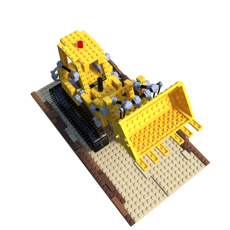
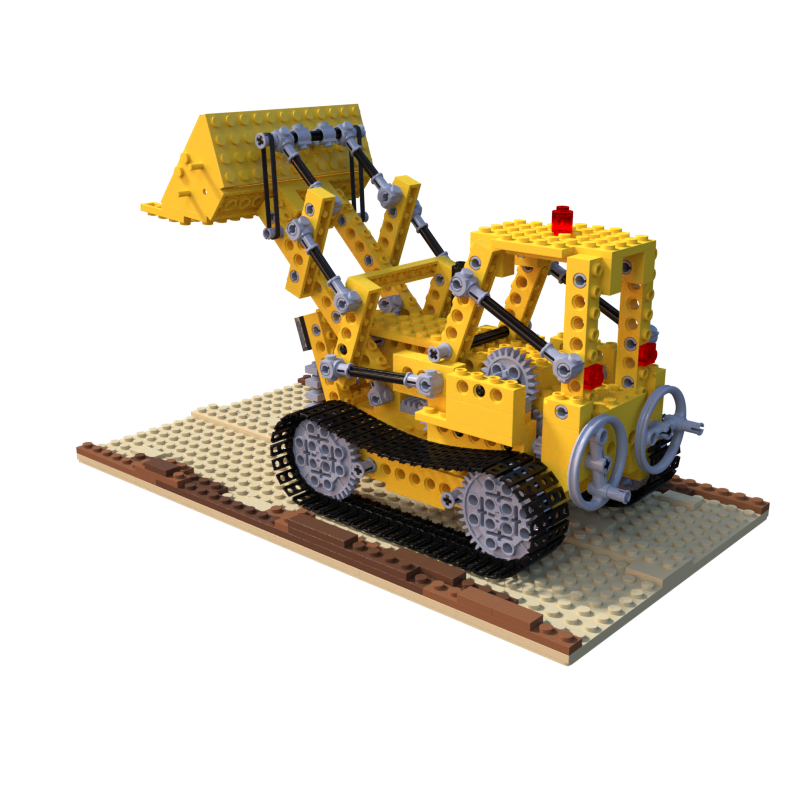
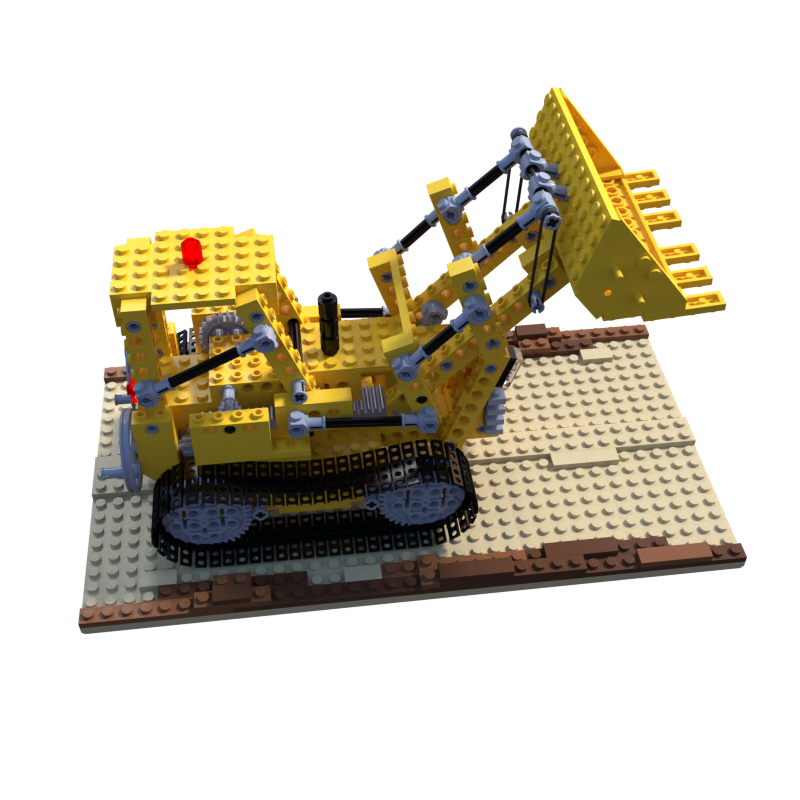
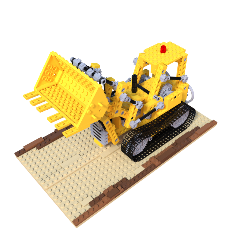
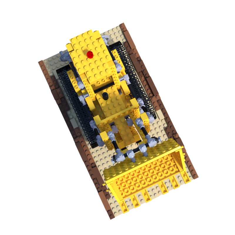
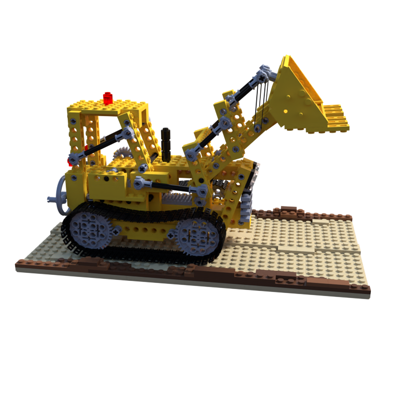
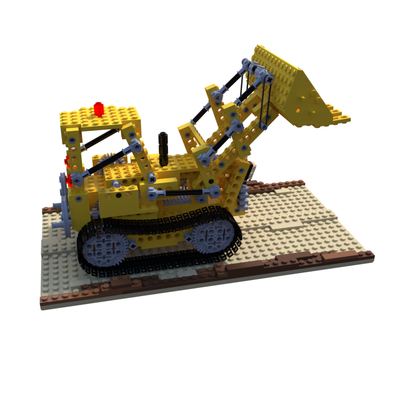
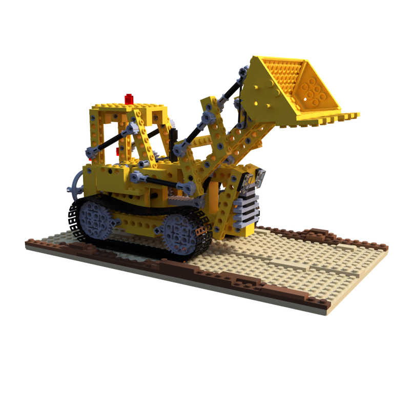
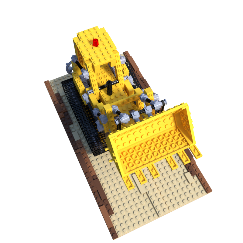
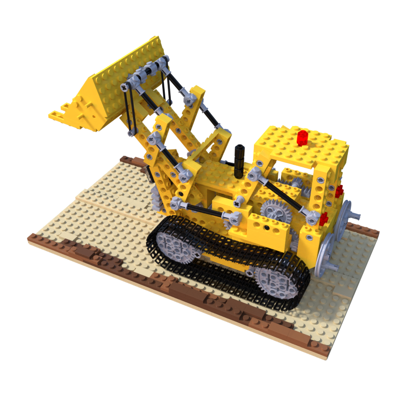
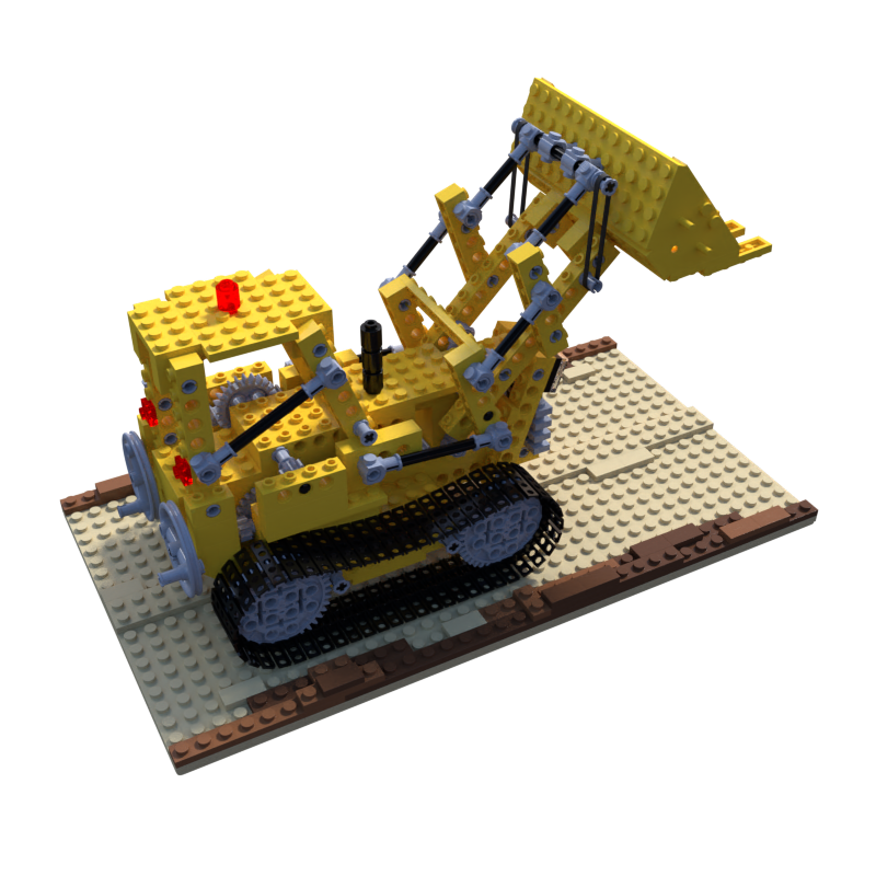
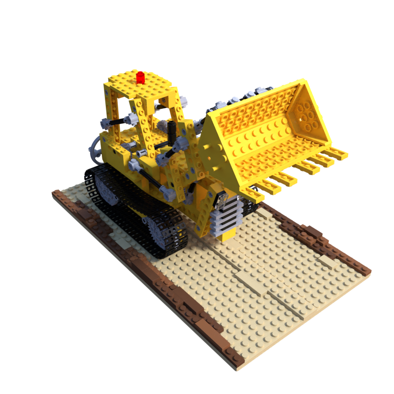
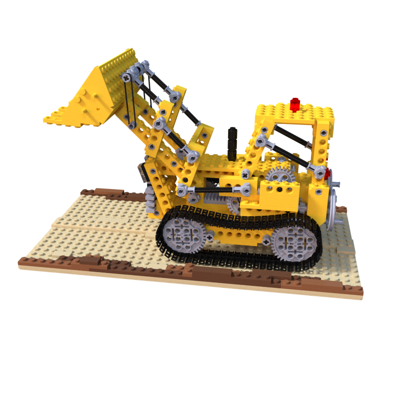
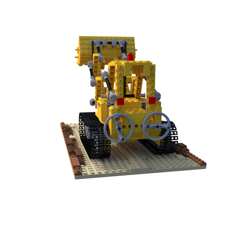
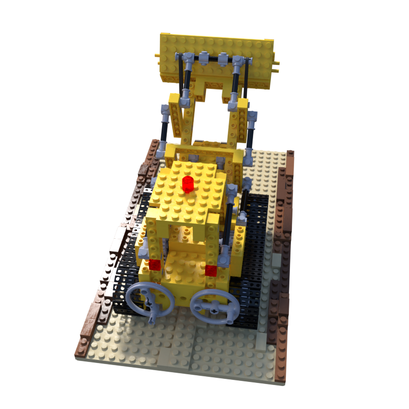
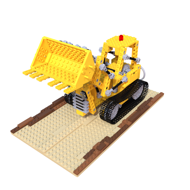
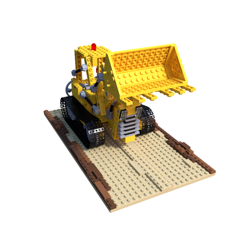
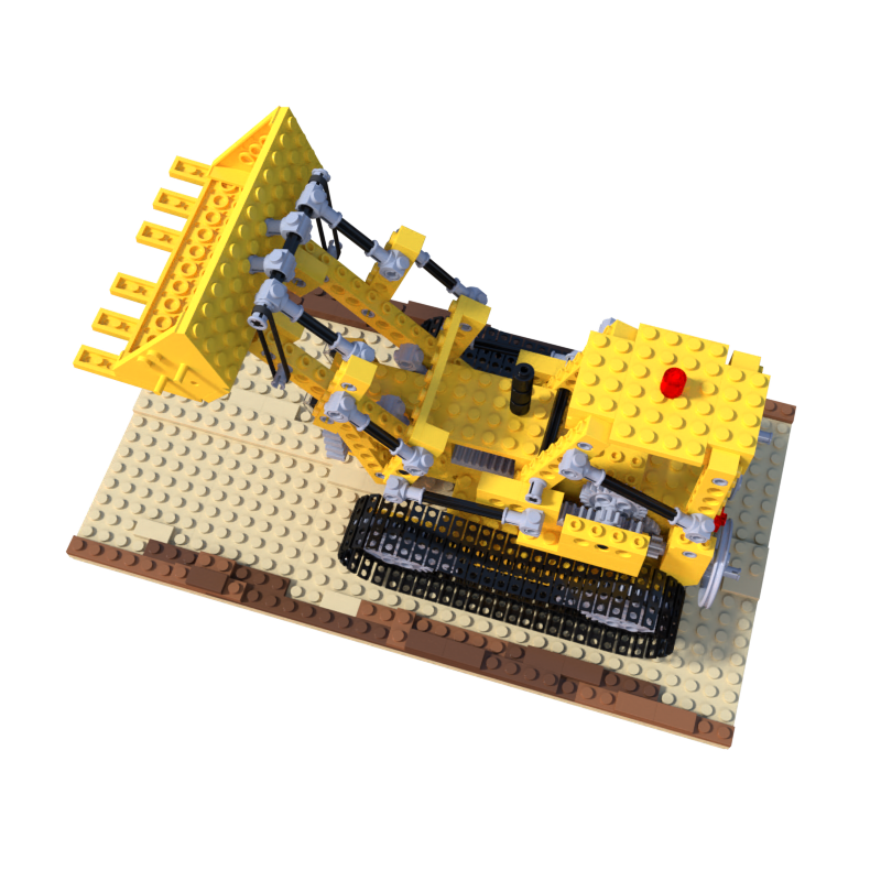
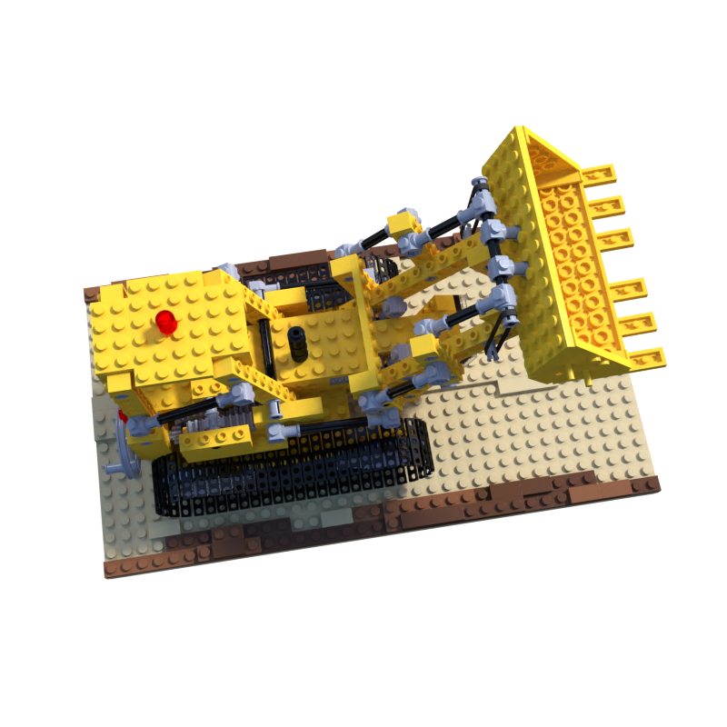
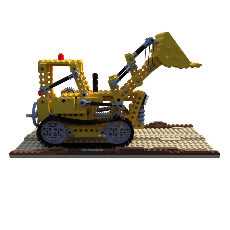
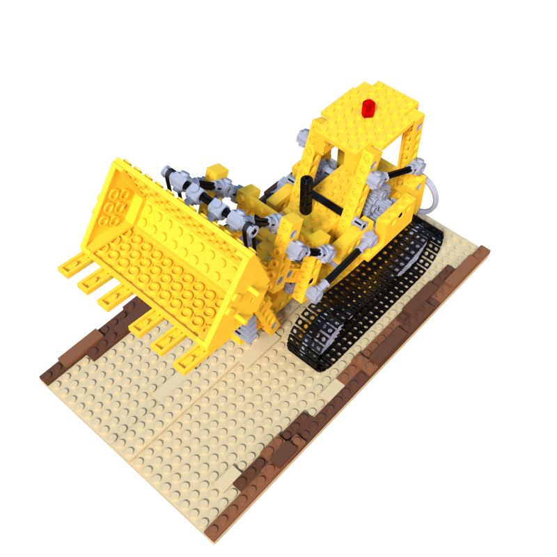
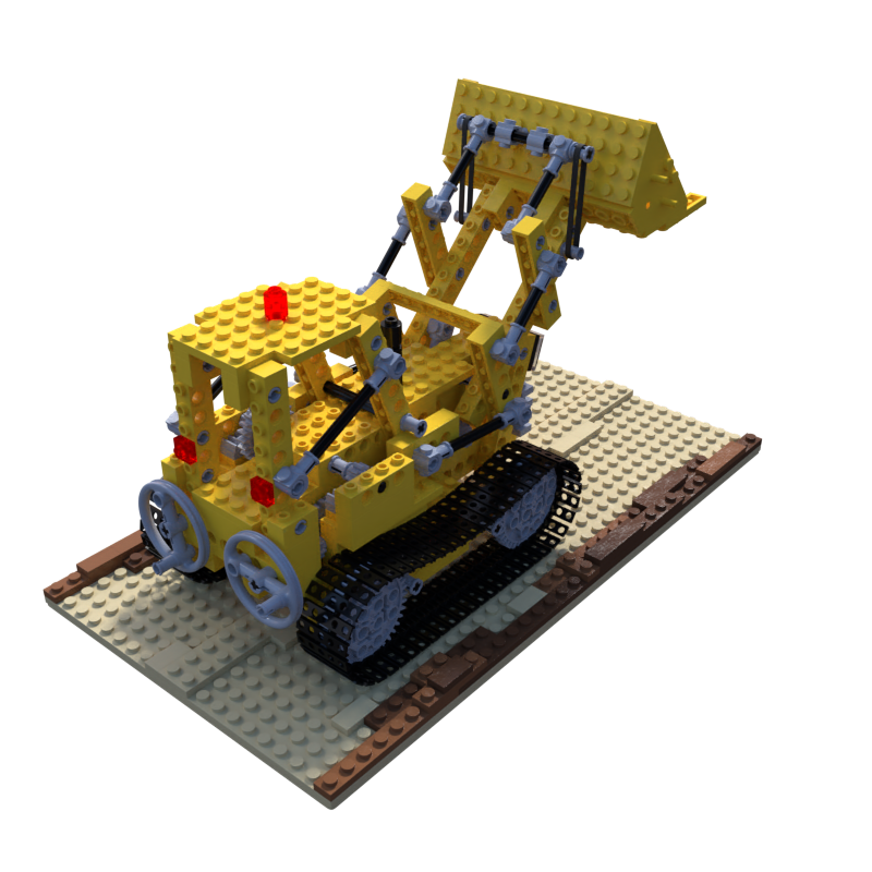
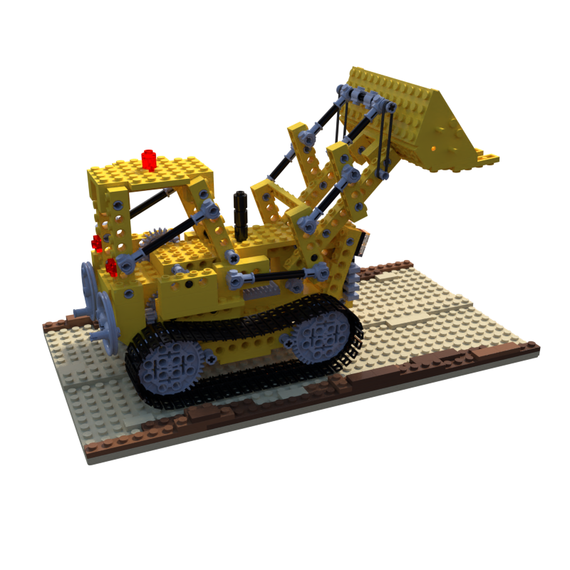
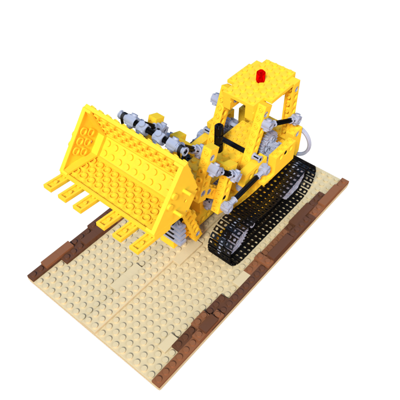
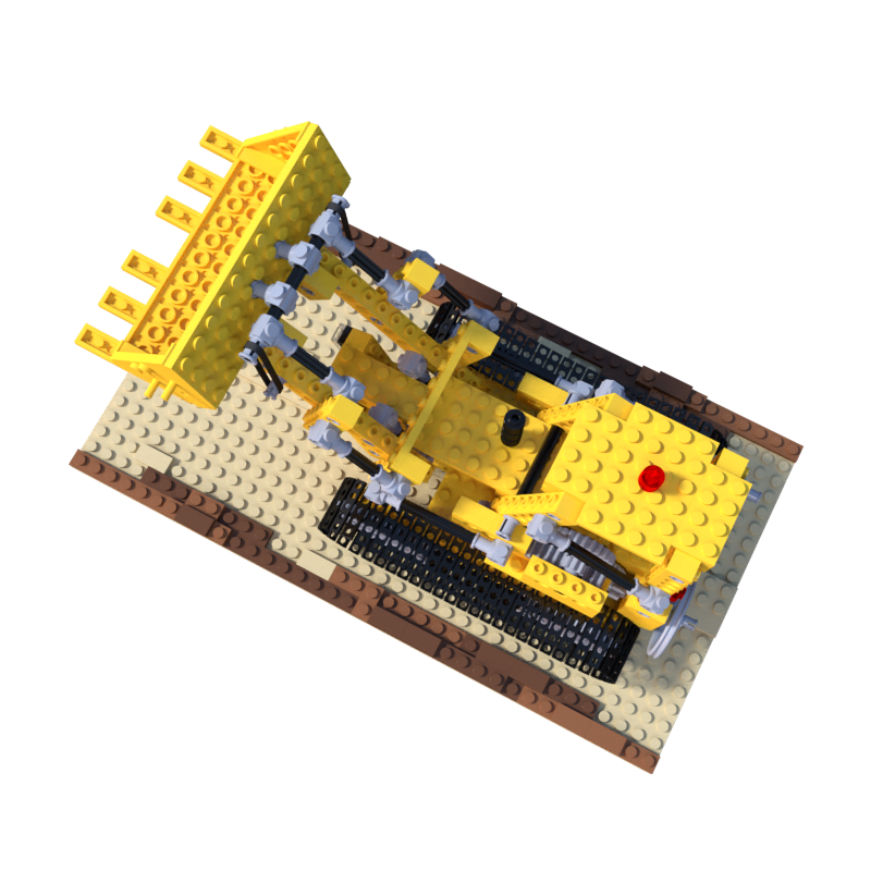
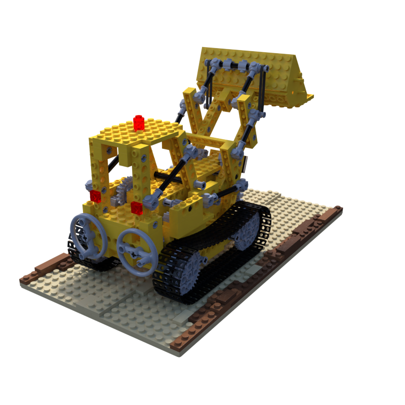
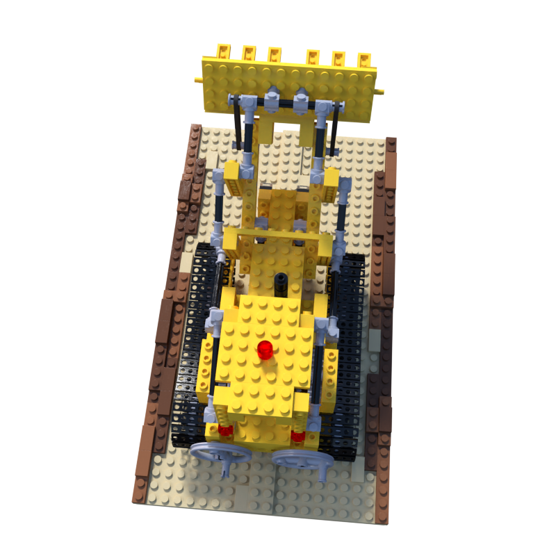
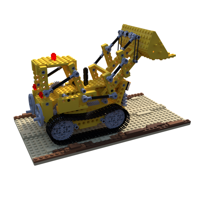
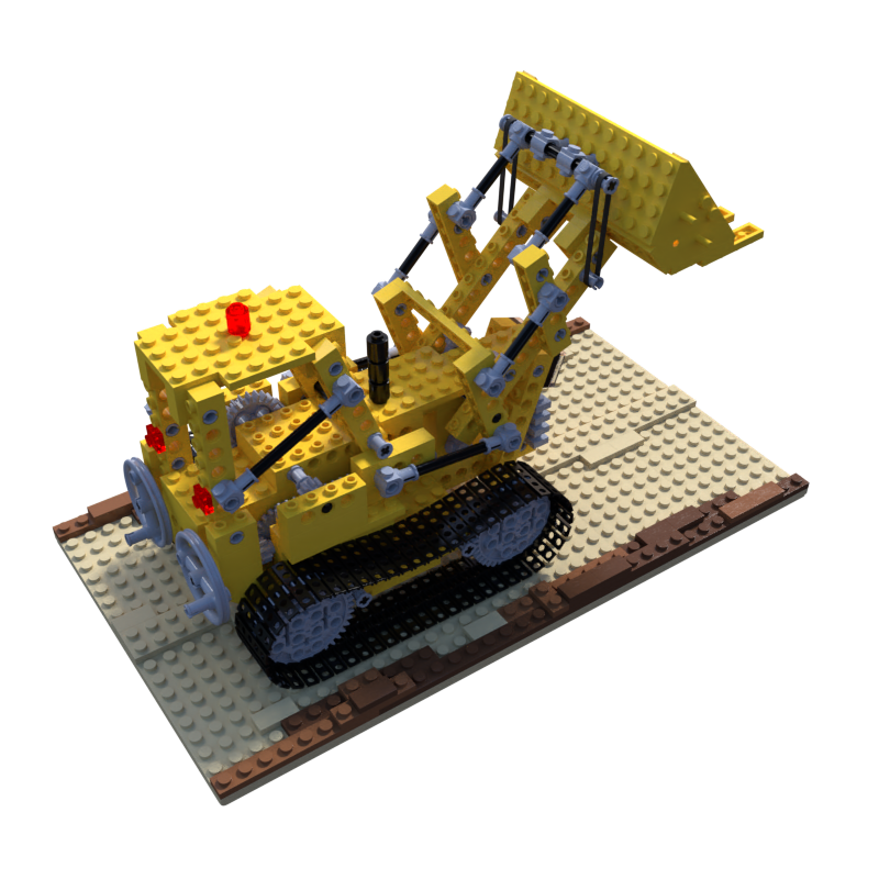
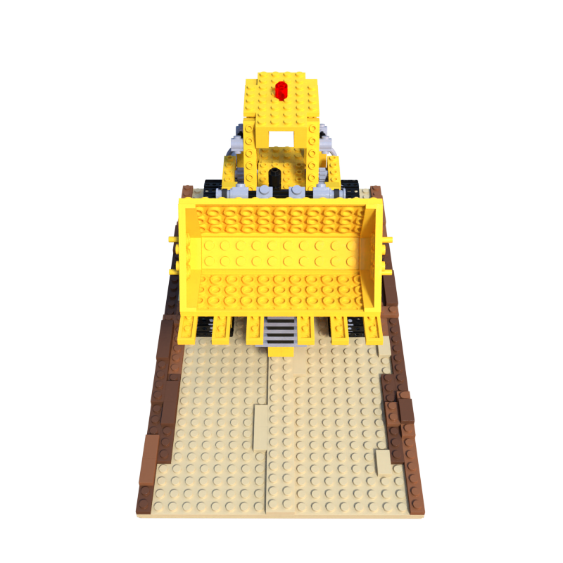
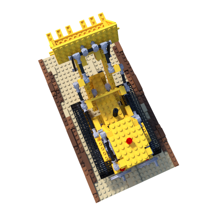
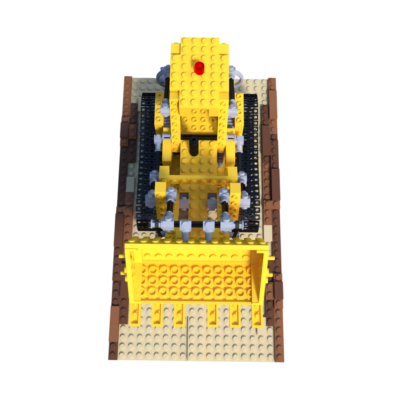
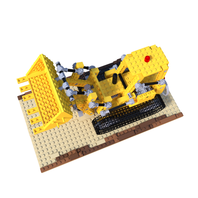
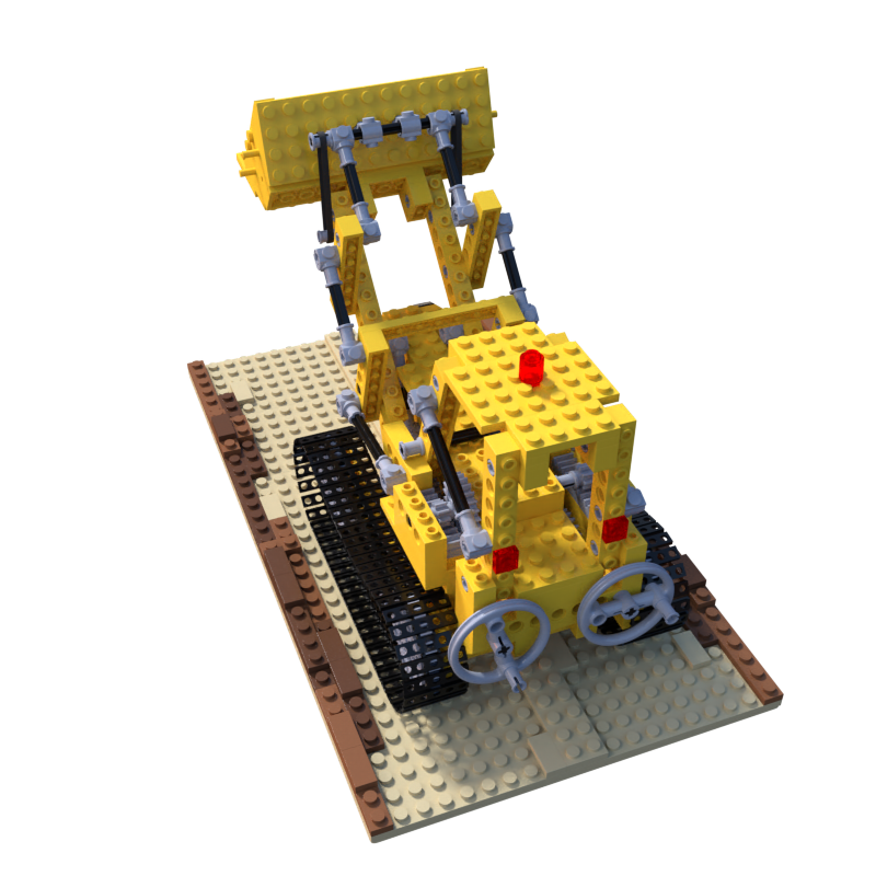
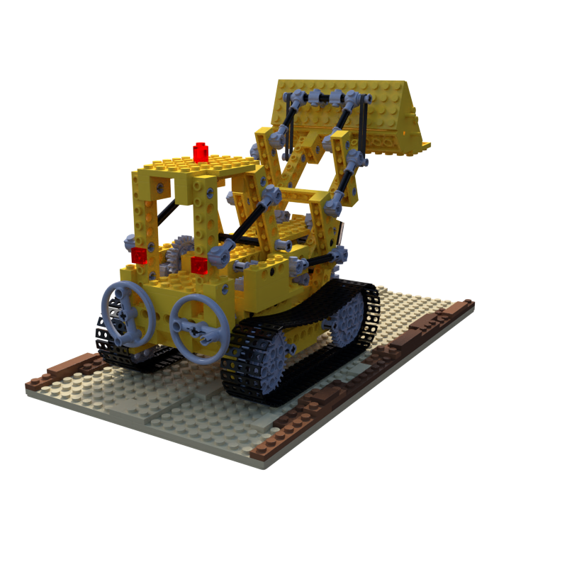
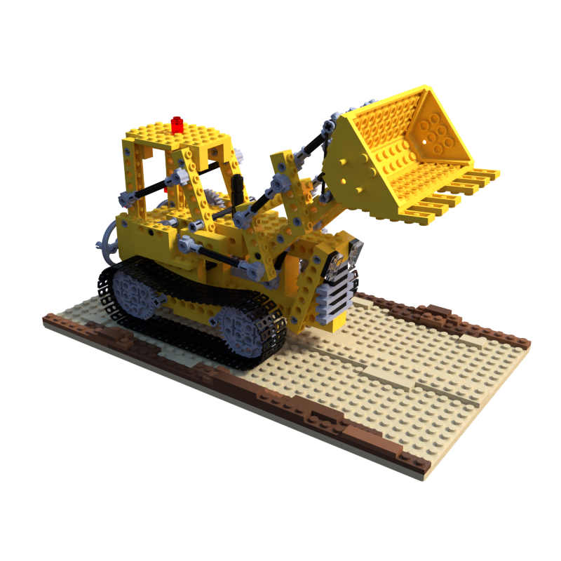
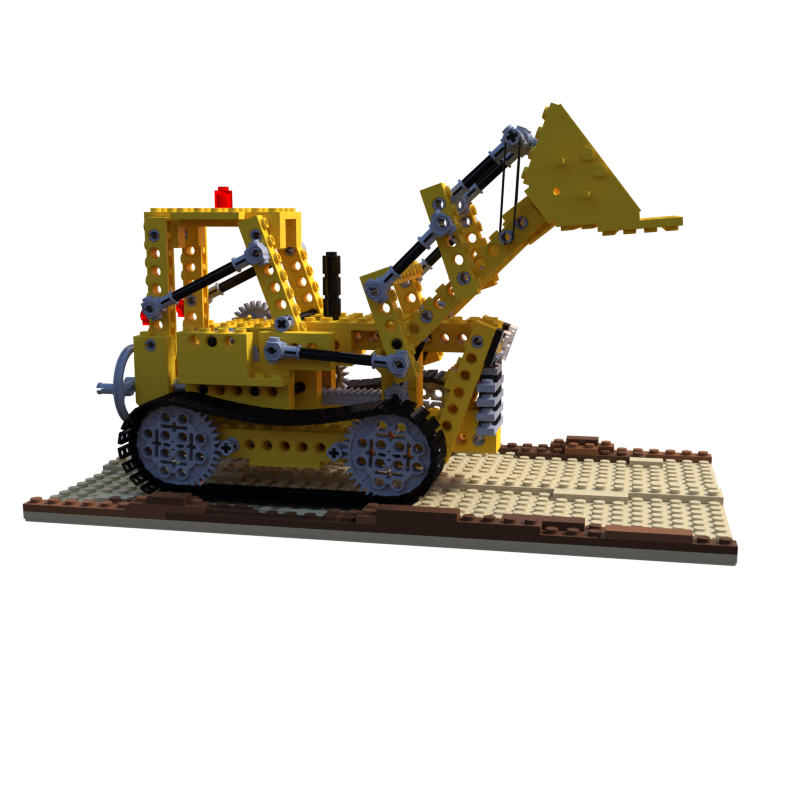
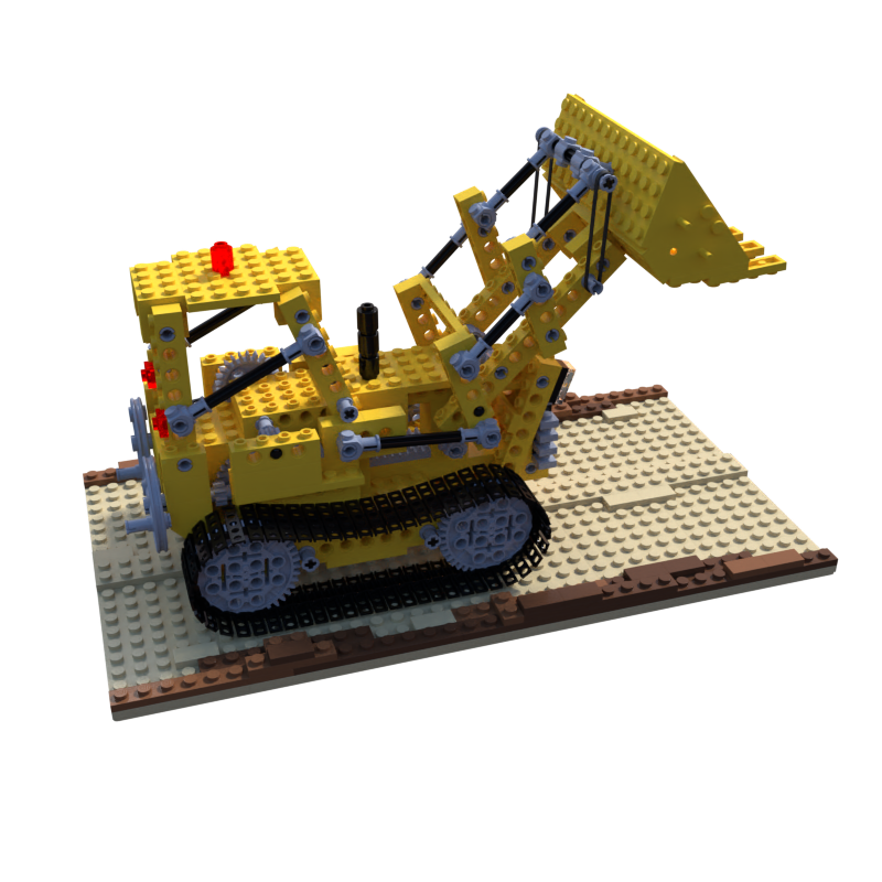
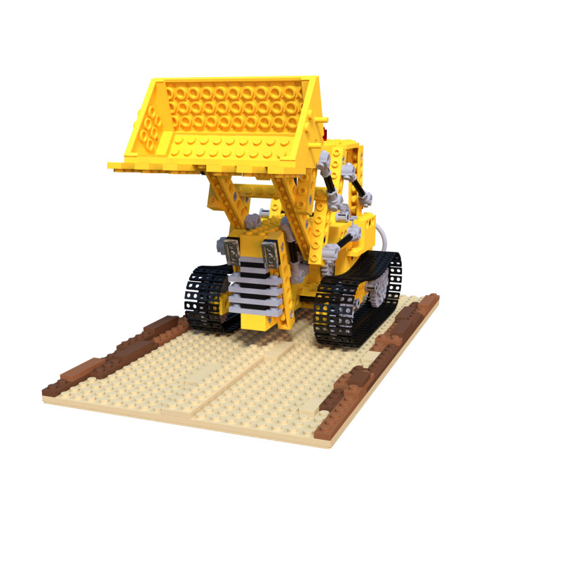
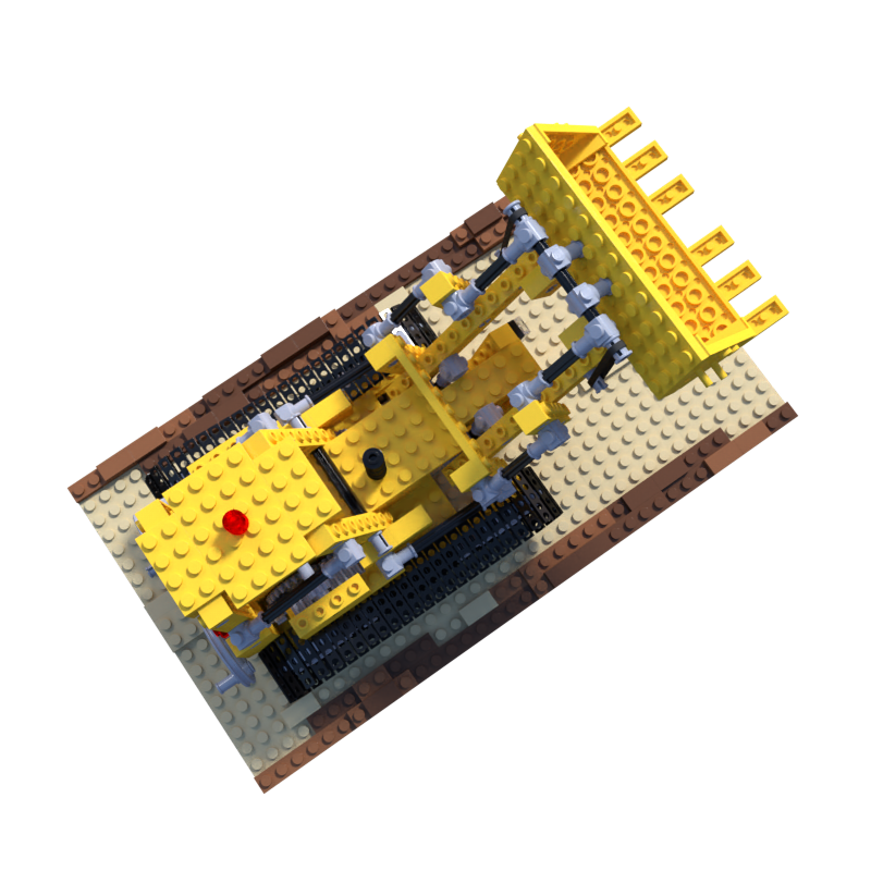
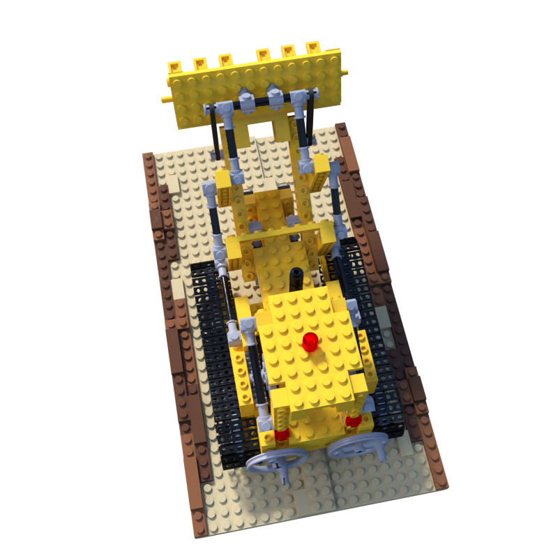
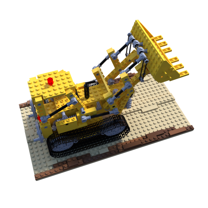
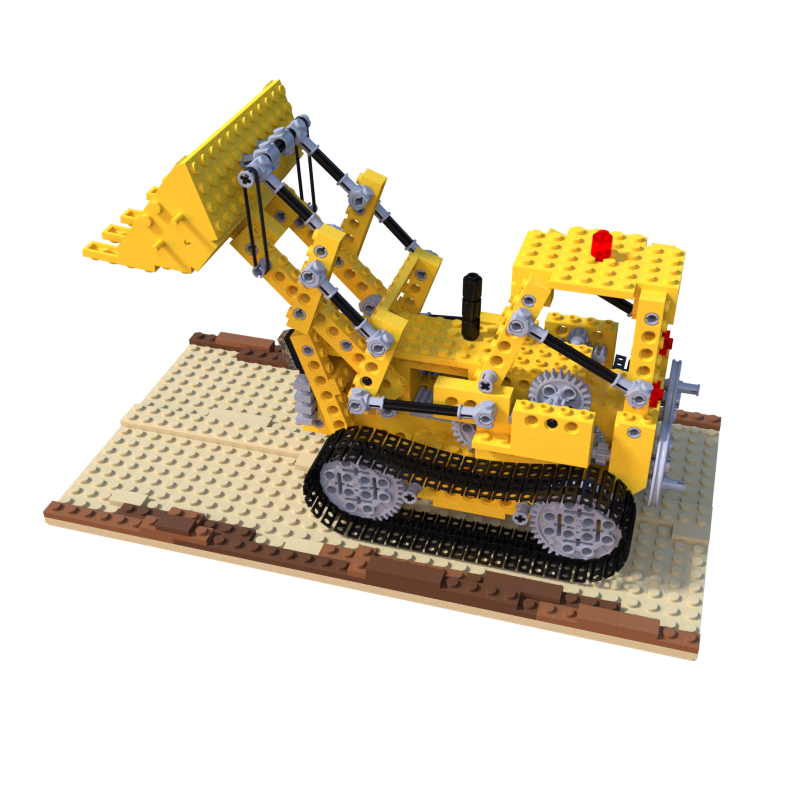
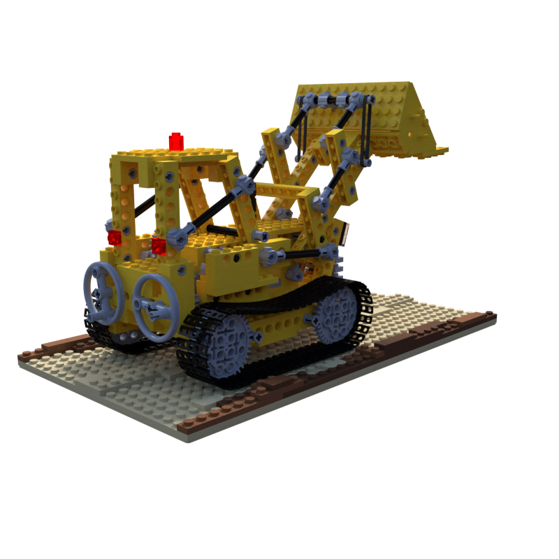
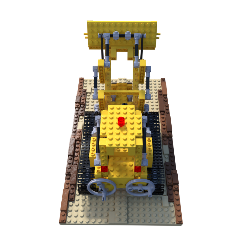
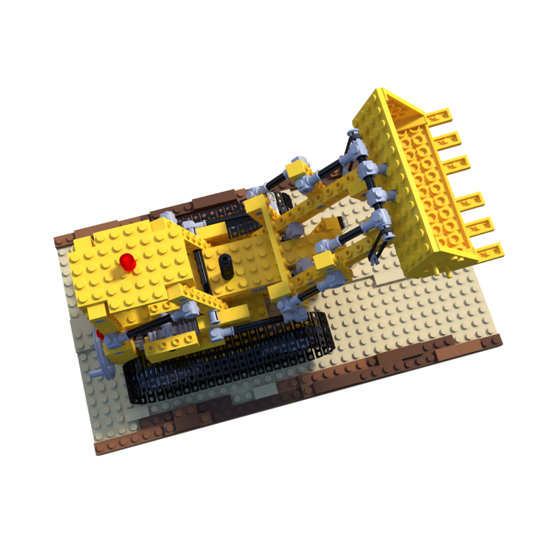
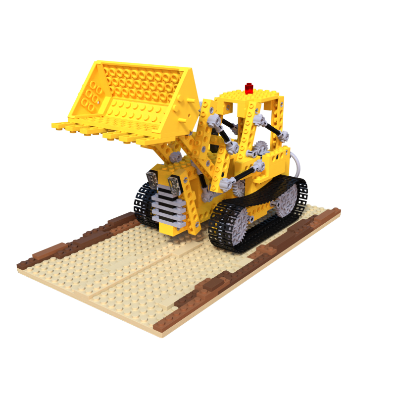
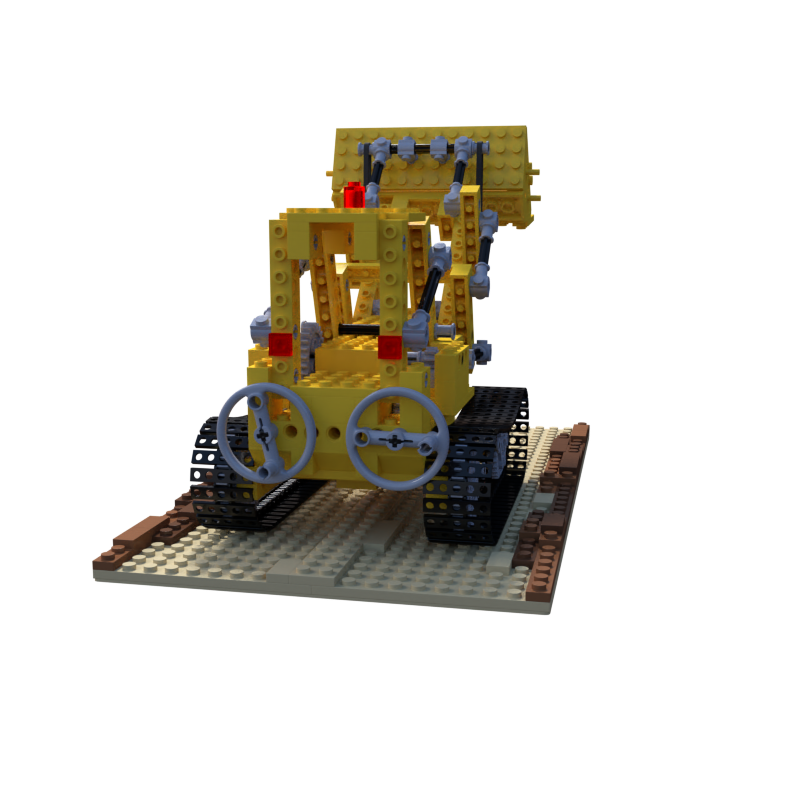
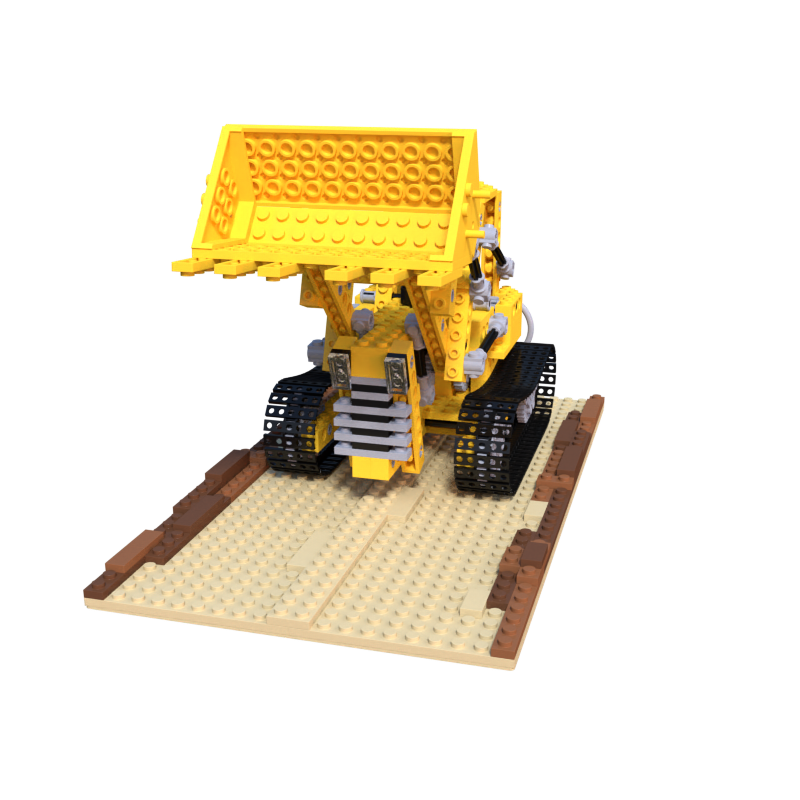
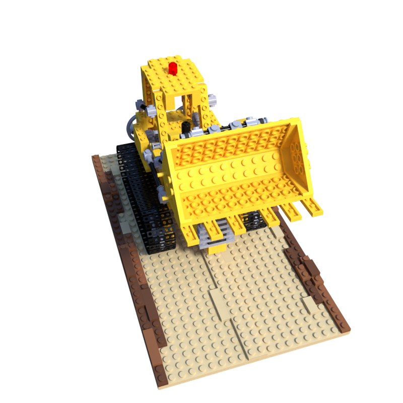
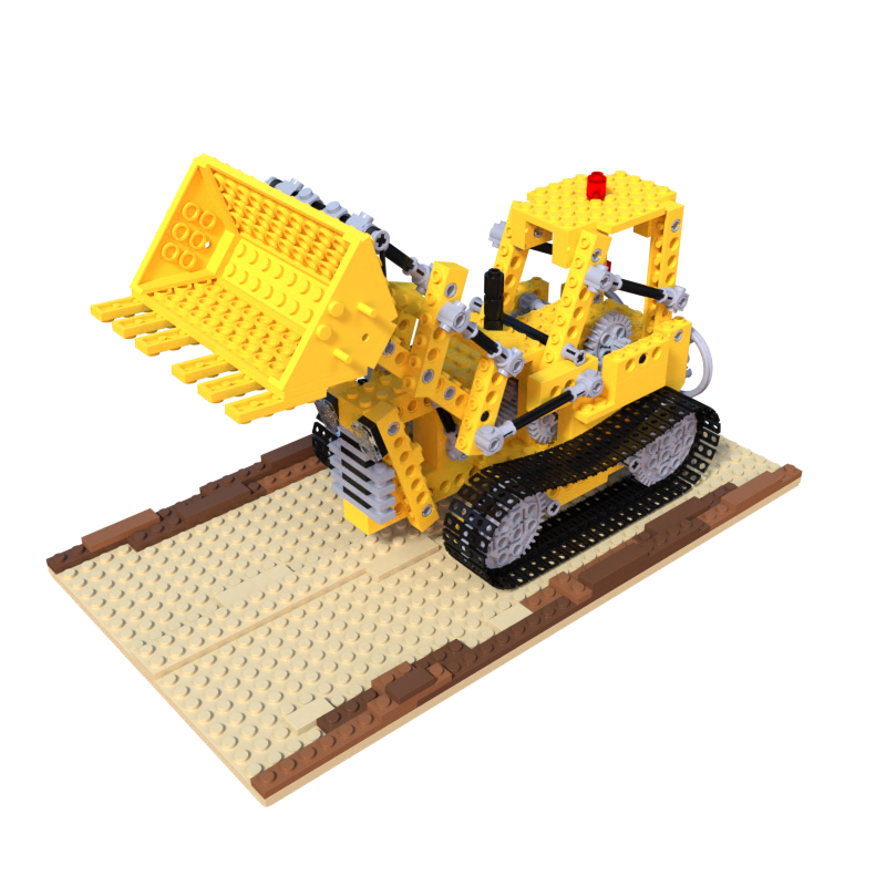
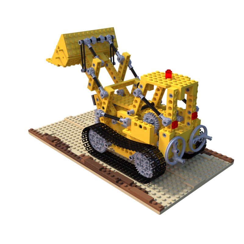
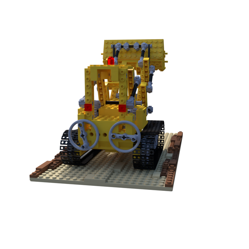
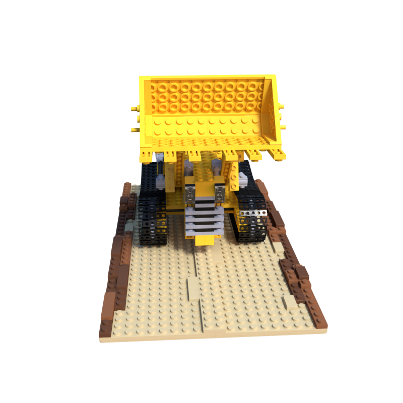
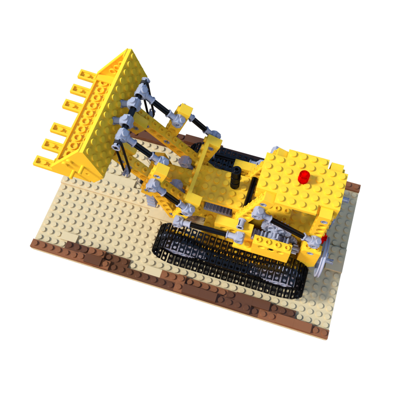
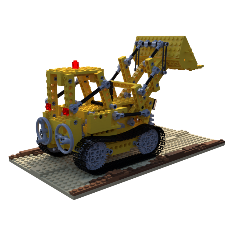
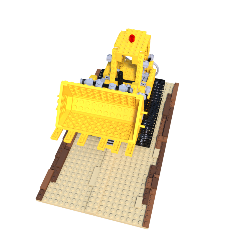
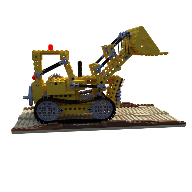
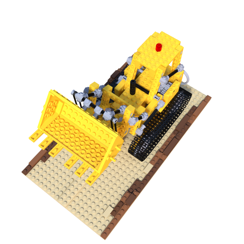
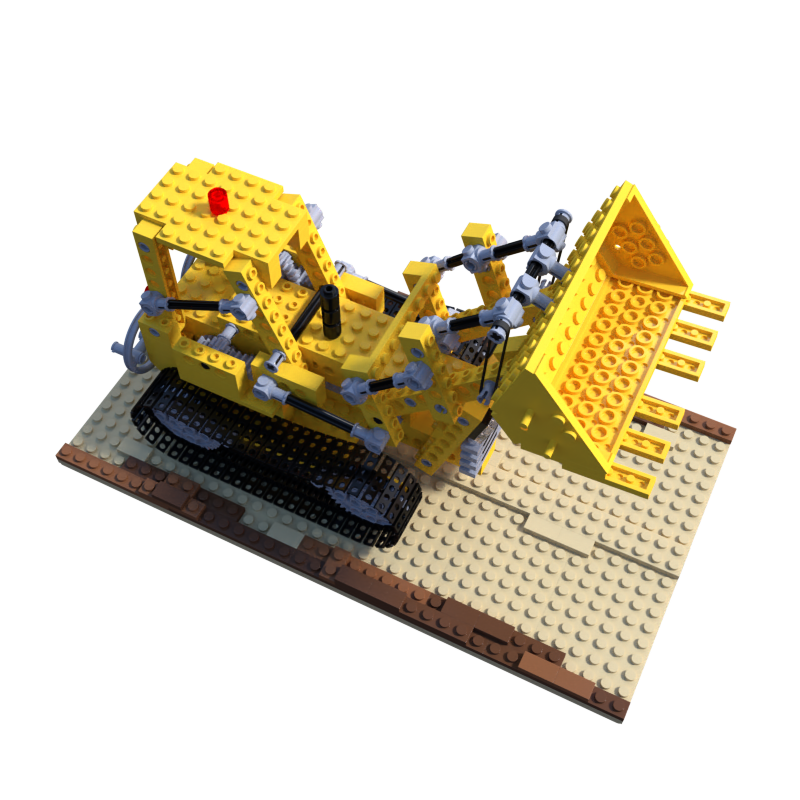
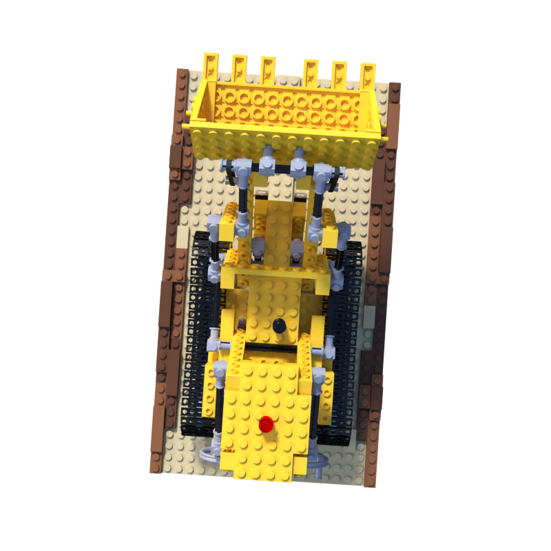
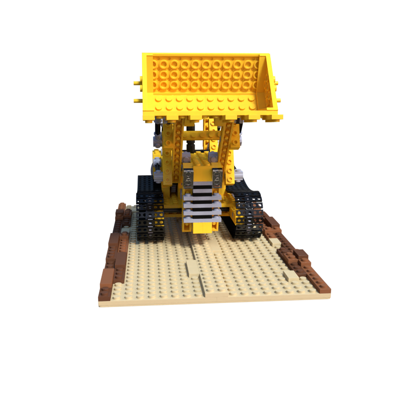
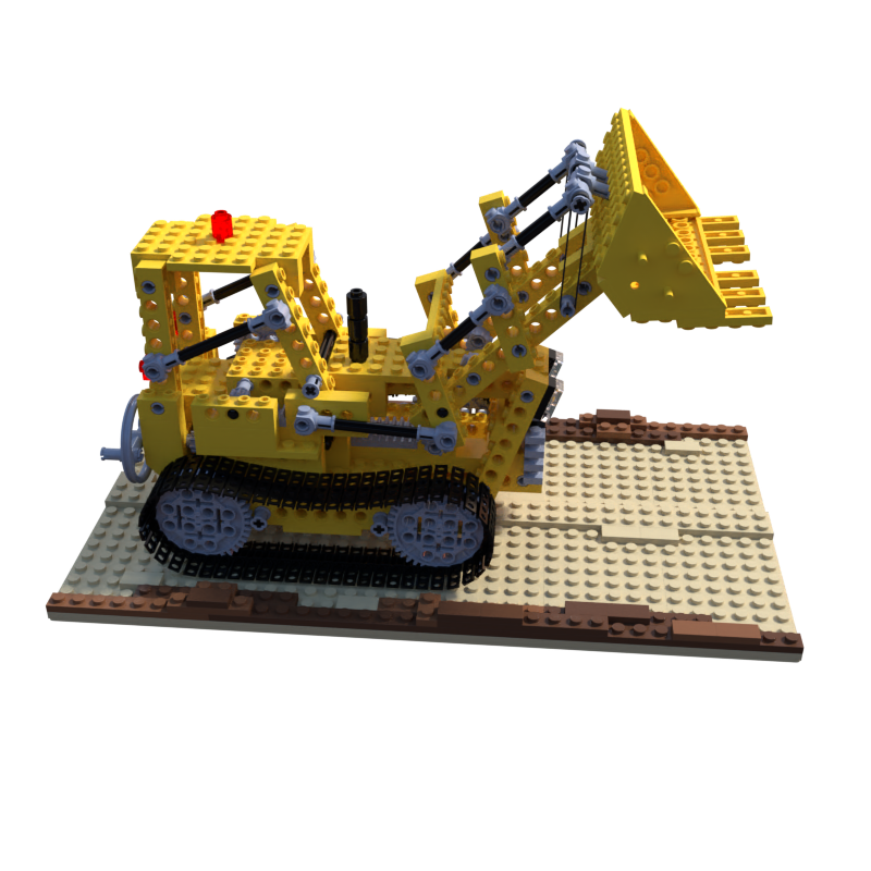
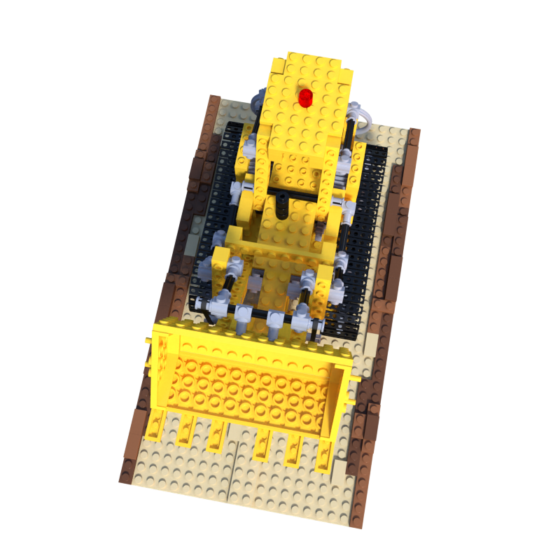
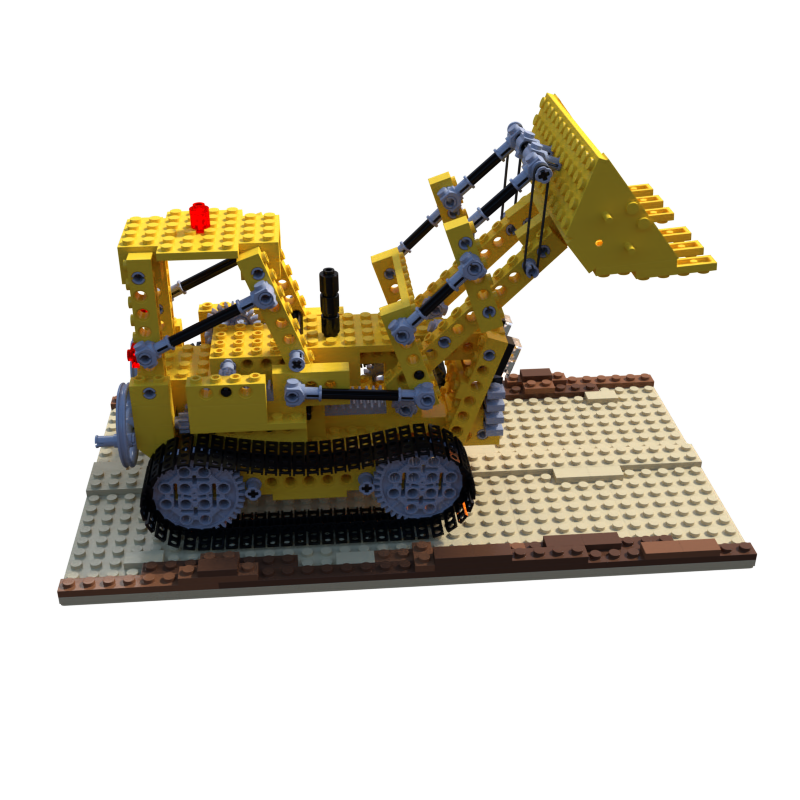
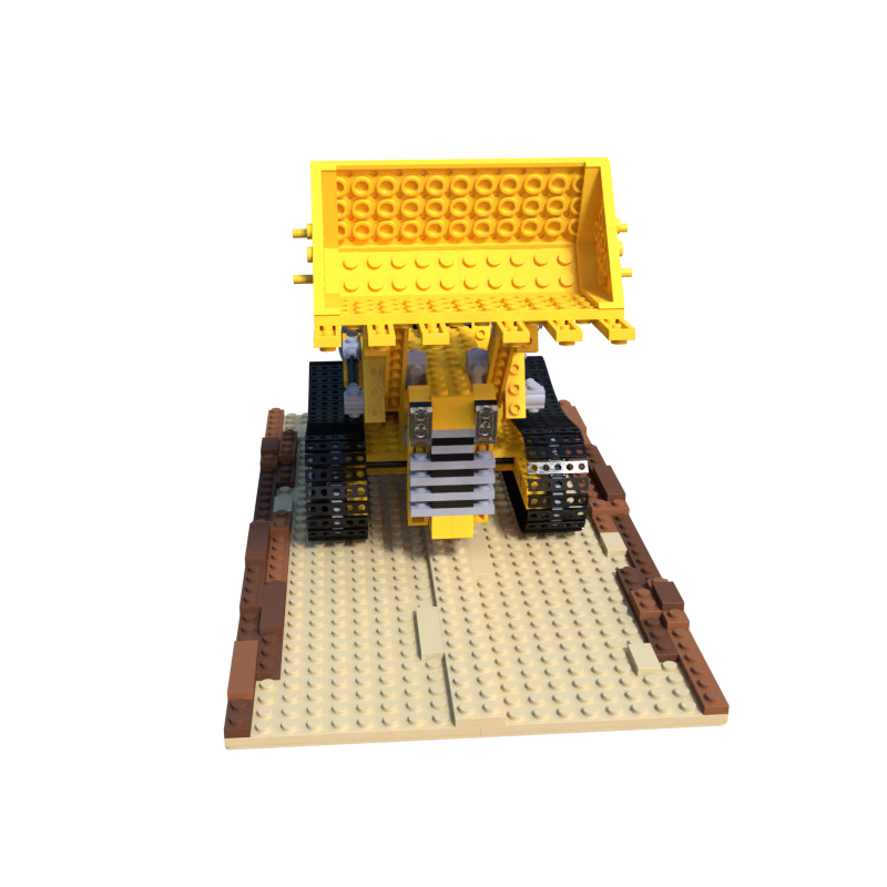
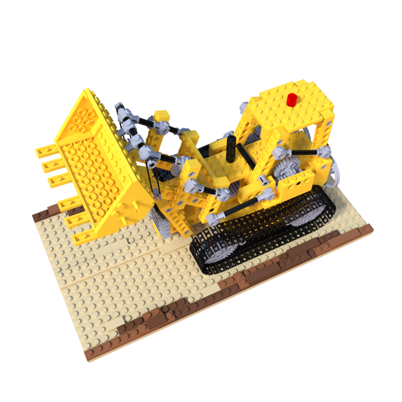
The model was trained on the Blender lego scene, the data for which can be found in the NeRF paper’s project page or downloaded from Kaggle - 100 training views of a lego bulldozer rendered from known camera poses on a hemisphere. Below are all 100 training images, the inputs NeRF was supervised on. No depth or 3D annotation were available during training, just pixels.

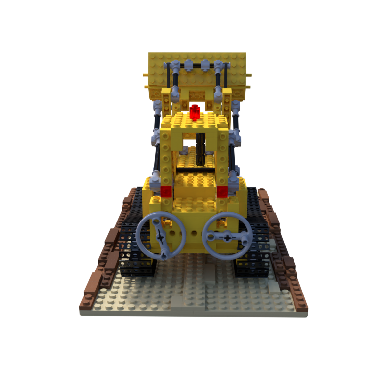
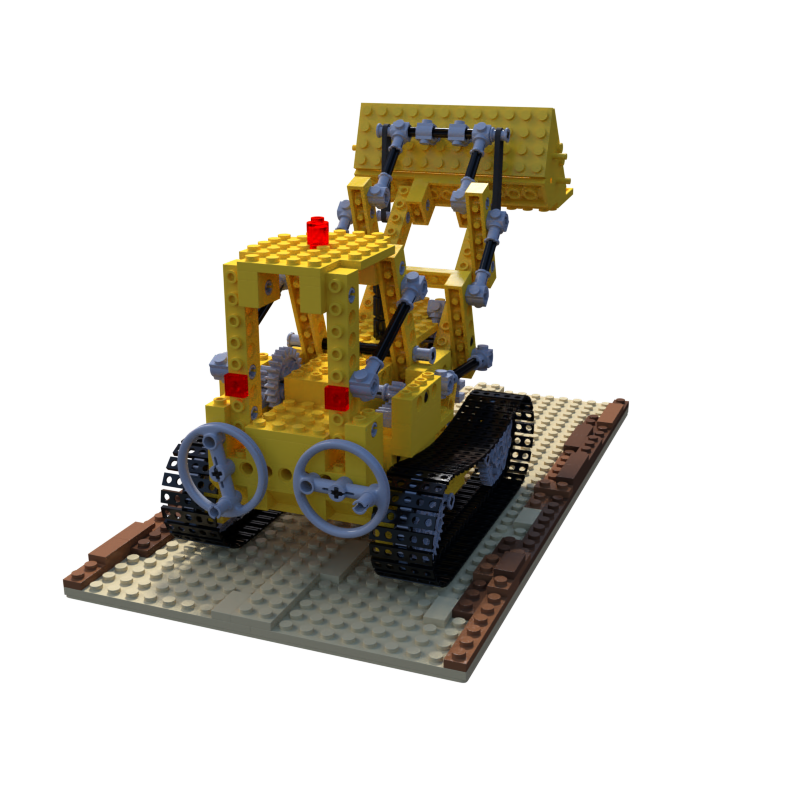
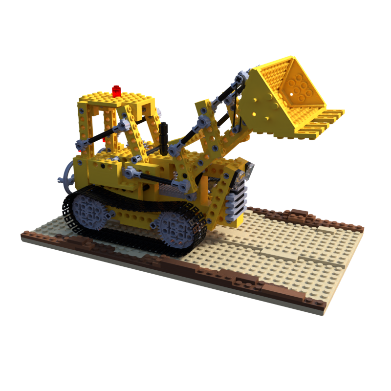
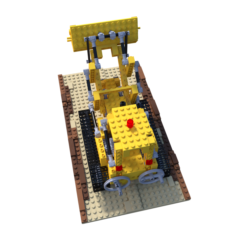
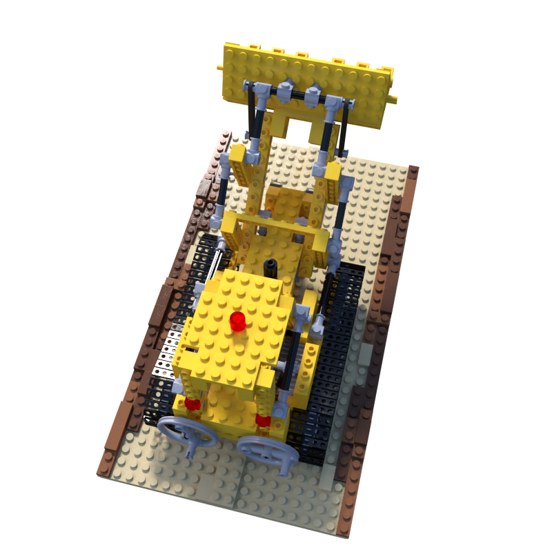
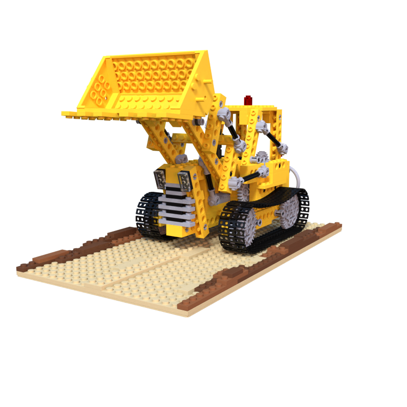
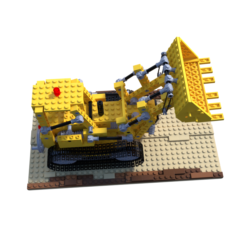
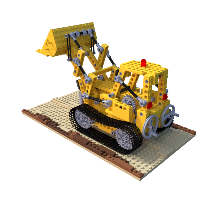
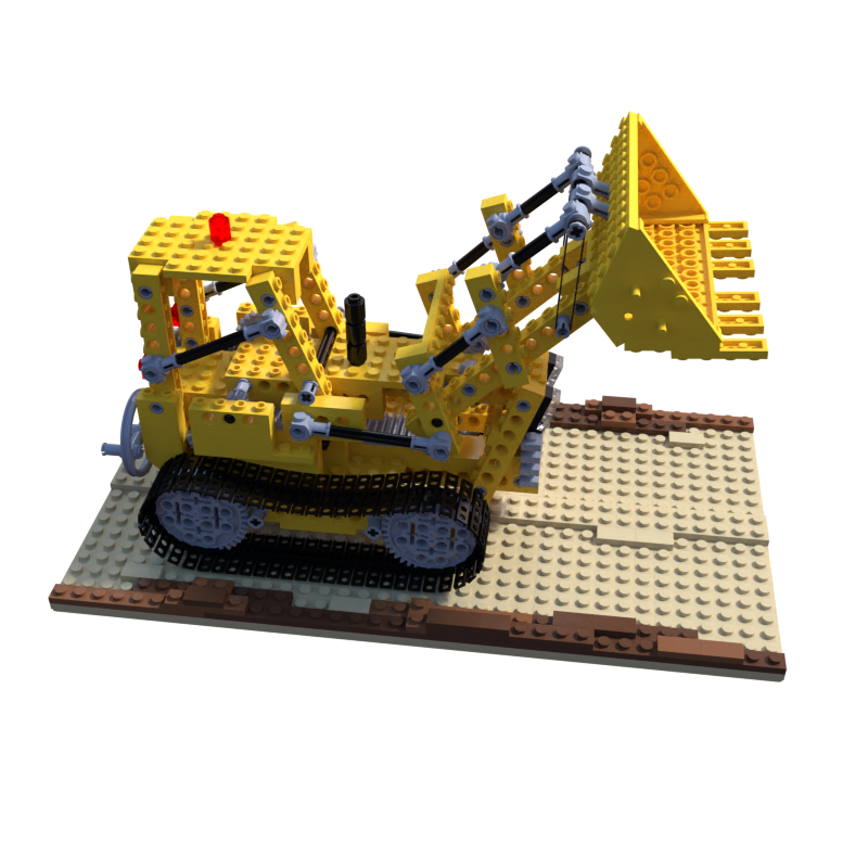
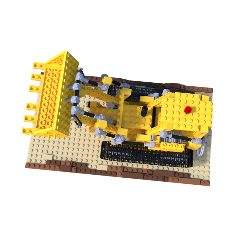
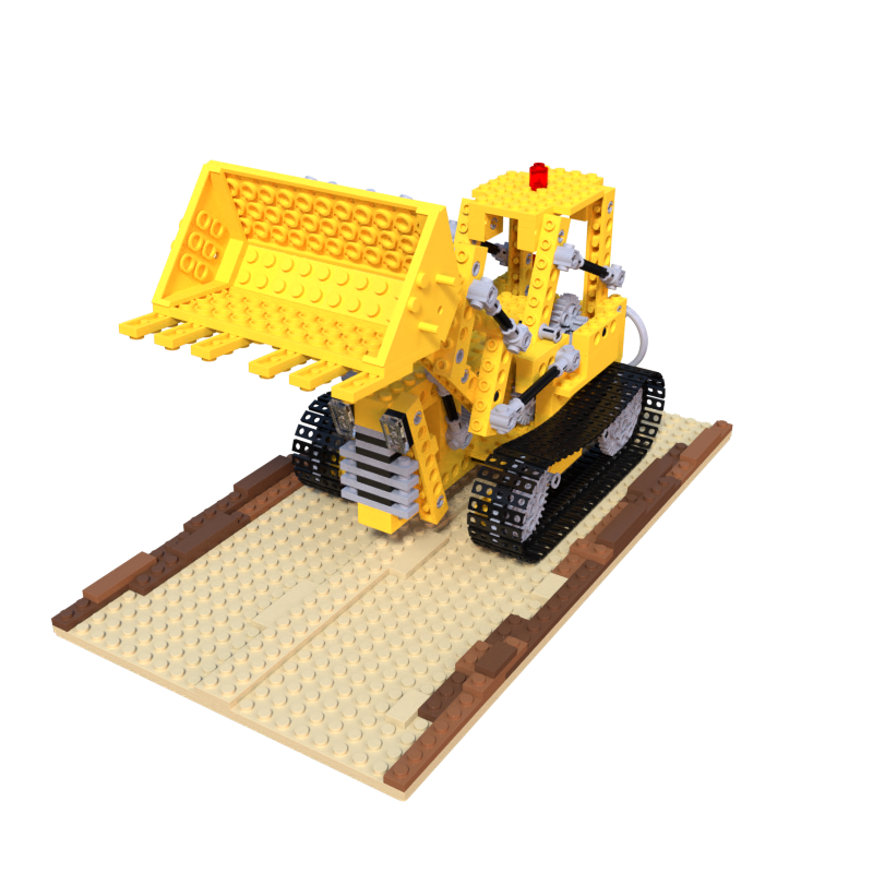
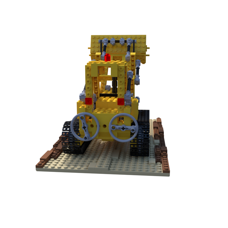
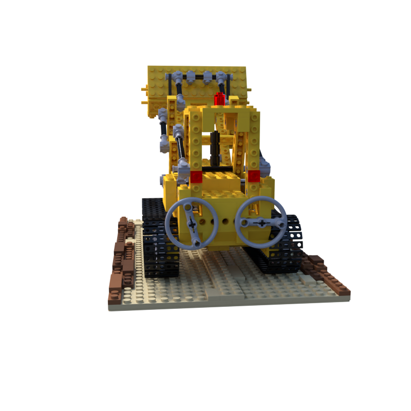
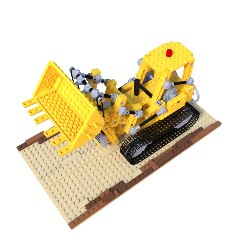
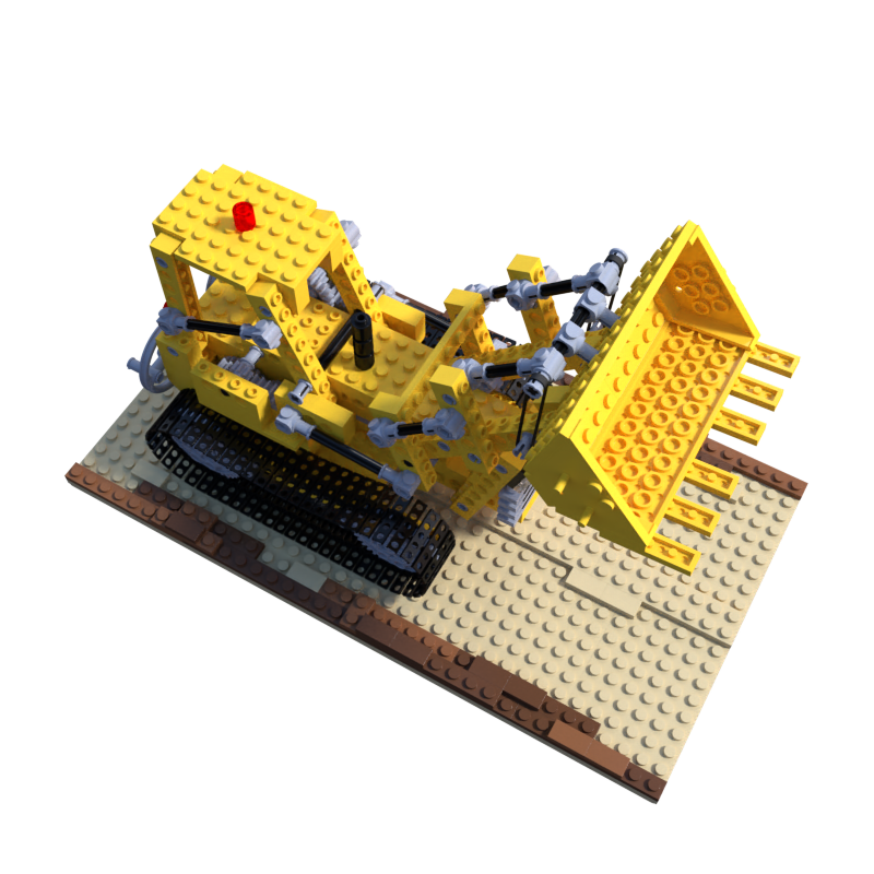
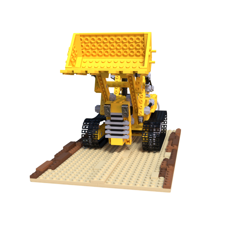
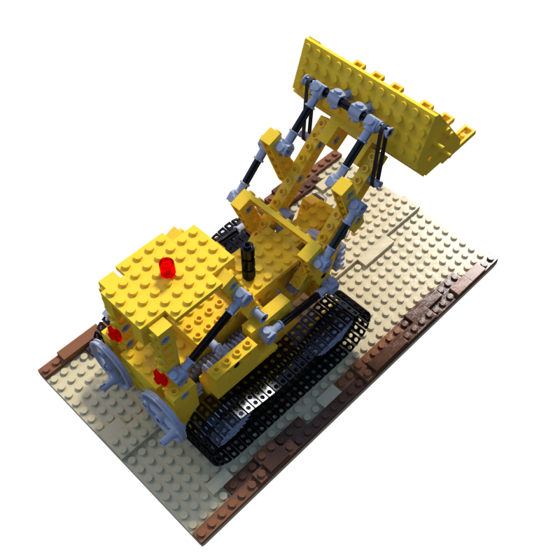
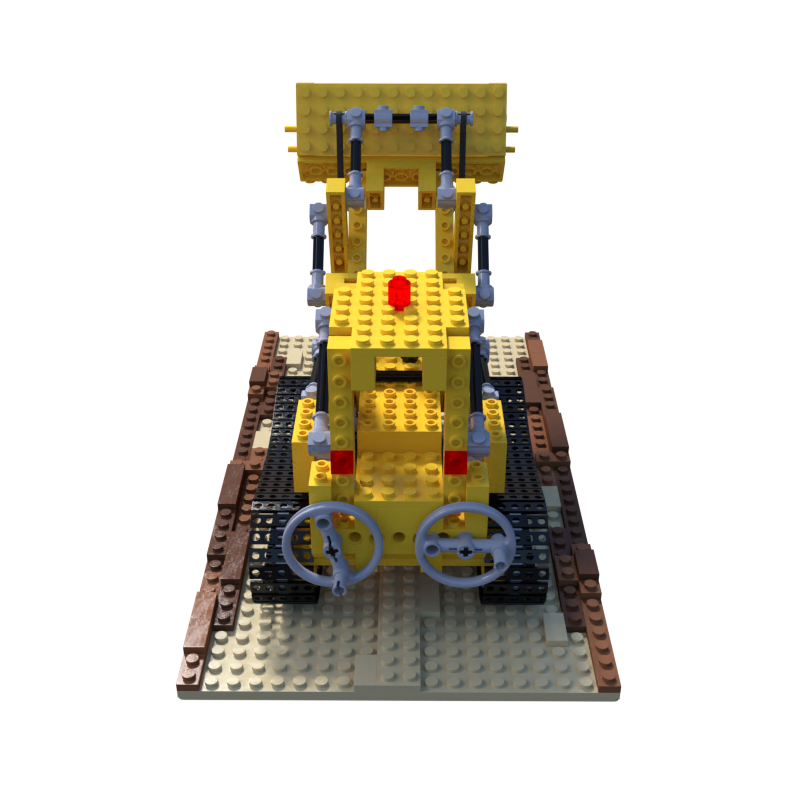
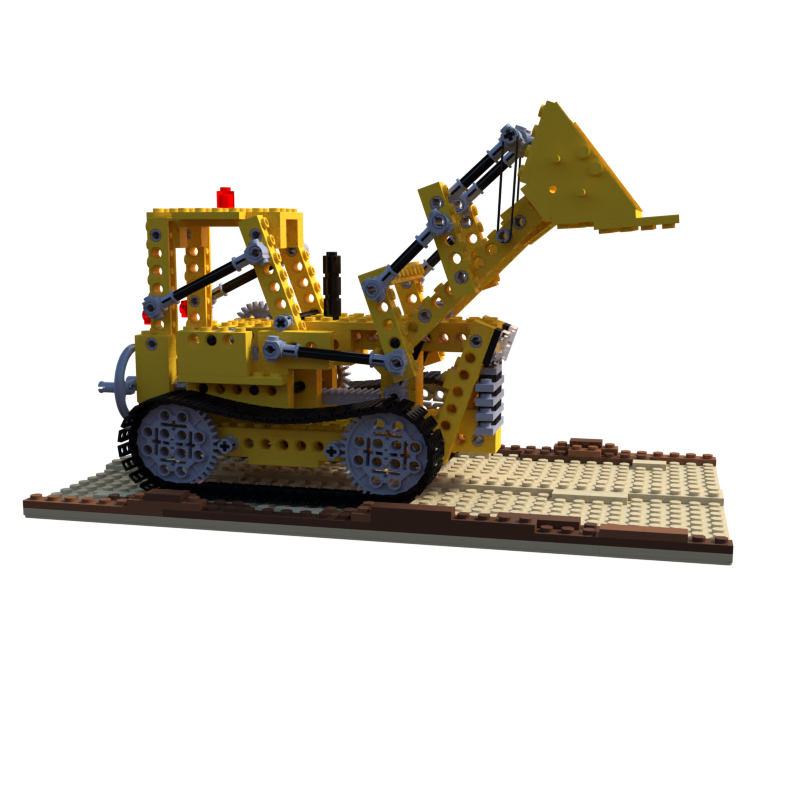
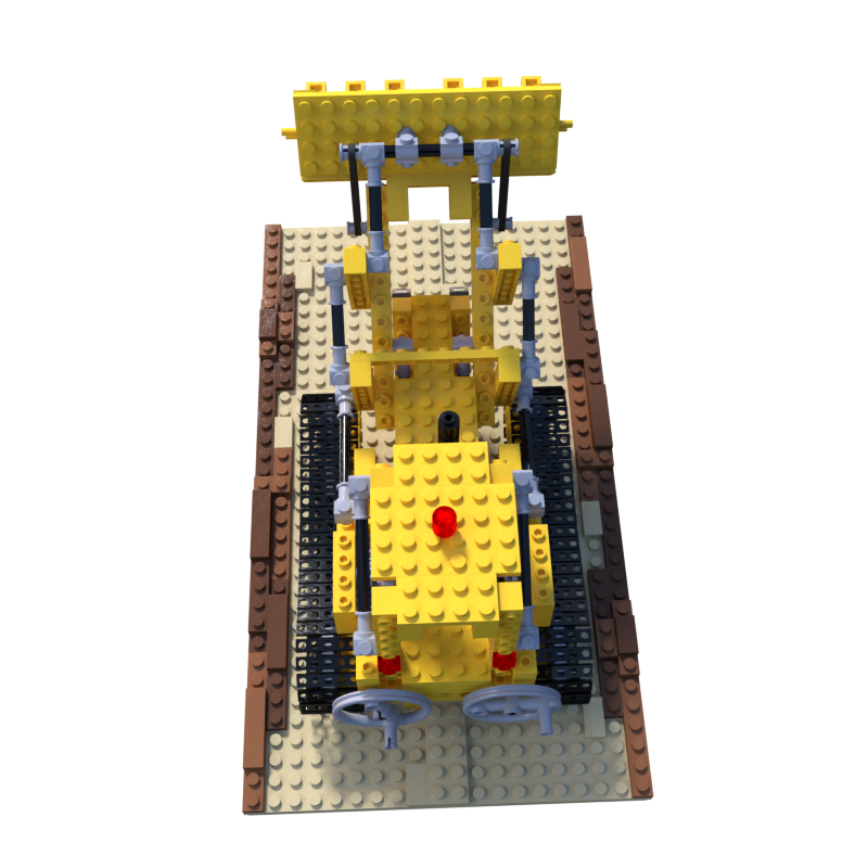
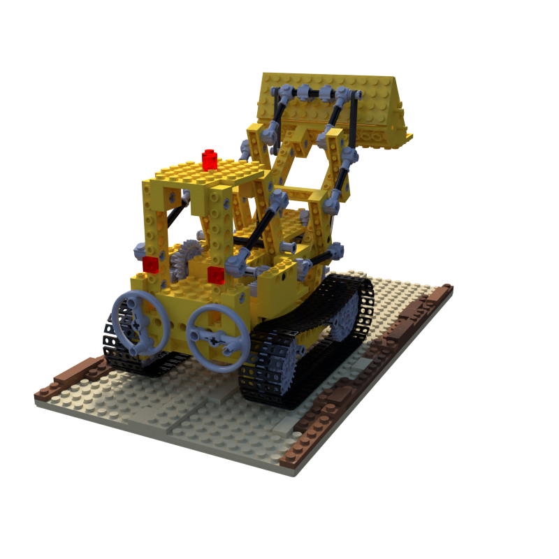
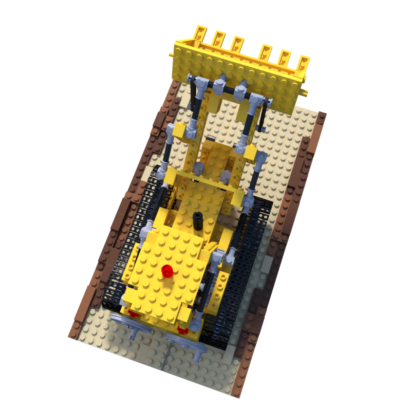
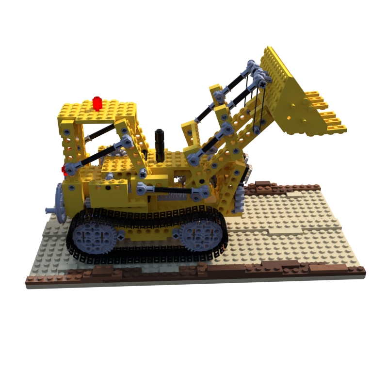
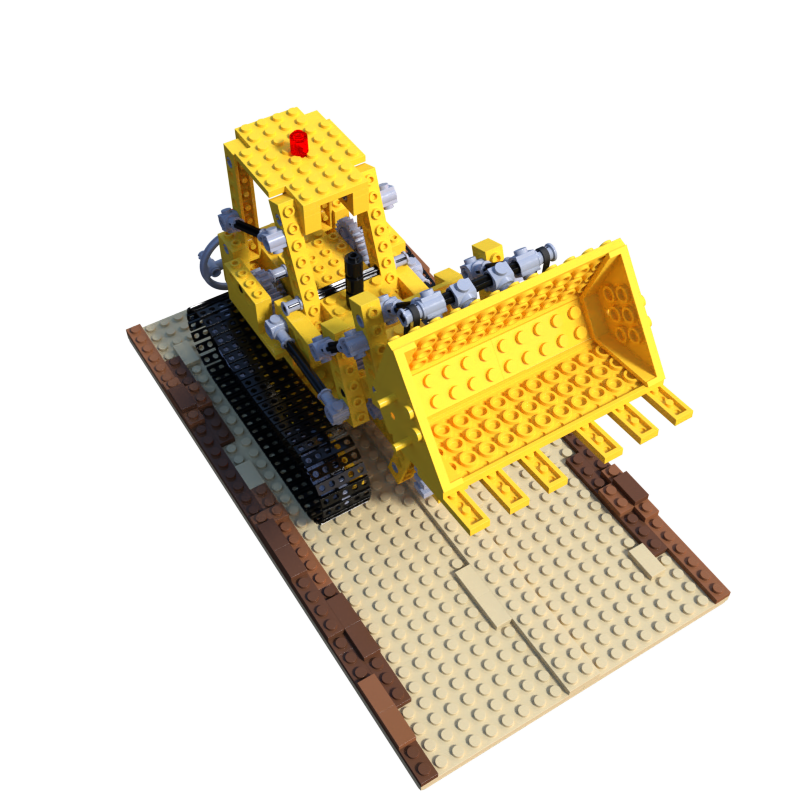
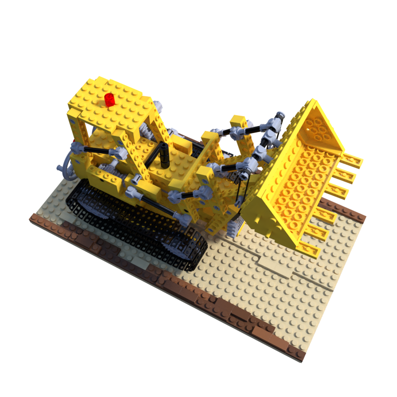
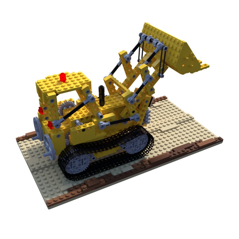
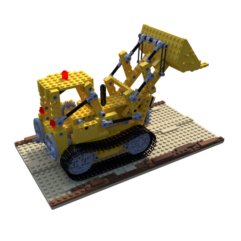
And here’s a novel view synthesis render at 100k iterations - 24 frames sweeping 360° around the scene, rendered from the EMA weights:

This is at the halfway point of training (100k of 200k iterations) since I was too impatient to wait for training to finish. The overall shape of the bulldozer is clearly there, and the model has learned 3D geometry pretty accurately from the 2D supervision alone. Some blurriness is still visible on fine details, which is expected at this stage. The view-dependent shading is already working: you can see the specular highlights shift as the camera rotates. The white background comes from white_bkgd=True: pixels where the ray exits the scene without hitting anything get assigned transmittance that adds up to white rather than black.

What’s notable here is that none of the frames in the video are in the training set. The 100 training images cover a fixed set of camera poses, but the video sweeps continuously around the scene at angles that were never seen during training. NeRF generalizes to these novel views because it learns a continuous volumetric representation of the scene, not a lookup table of images. Any new camera pose just queries the same MLP at new 3D sample points along new rays, and the rendering equation produces a pixel color. This is novel view synthesis, the ability to render a scene from an arbitrary viewpoint given only a sparse set of input photos.

Section 4: Recap & what’s next

NeRF represents a scene as a neural function from position and direction to color and density, supervised purely from 2D pixels via differentiable volume rendering. No explicit 3D supervision needed.

Main limitations: slow training (hundreds of thousands of iterations) and slow inference (rendering a single frame requires evaluating the MLP at millions of 3D points: ~192 samples per ray, across every pixel). A lot of follow-up work, such as Instant-NGP, Mip-NeRF, 3D Gaussian Splatting, addresses these bottlenecks directly.

In the next post, we’ll look at Instant-NGP (paper, Github) for a significant speedup!

Useful Resources

1. Theory

NeRF paper: Representing Scenes as Neural Radiance Fields for View Synthesis - Mildenhall et al., 2020.
NeRF Explosion 2020 - Frank Dellaert’s overview of the NeRF landscape.

2. Code

bmild/nerf - the official TensorFlow implementation from the authors.
yenchenlin/nerf-pytorch - clean PyTorch port.

Citation

Le, Nhi. "Spatial Intelligence - Part 1: NeRF". halannhile.github.io (May 2026). https://halannhile.github.io/posts/nerf/

BibTeX:

@article{nhi2026nerf,
  title = {Spatial Intelligence - Part 1: NeRF},
  author = {Nhi},
  journal = {halannhile.github.io},
  year = {2026},
  month = {May},
  url = "https://halannhile.github.io/posts/nerf/"
}

Table of Contents#

Section 1: Theory#

1. What problem are we solving?#

2. The NeRF representation#

3. Volume rendering#

4. Optimizing a Neural Radiance Field#

4.1 Positional encoding#

4.2 Hierarchical volume sampling#

5. Training#

Section 2: Code#

1. Overview#

2. Ray generation#

3. Positional encoding#

4. The NeRF network#

5. Volume rendering in code#

6. Hierarchical sampling#

7. Training loop#

What to look for during training#

8. MPS optimizations#

1. Pre-cached rays#

2. bfloat16 AMP#

3. EMA (Exponential Moving Average)#

4. torch.compile#

5. LR warmup#

Section 3: Results#

Section 4: Recap & what’s next#

Useful Resources#

1. Theory#

2. Code#

Citation#

Table of Contents

Section 1: Theory

1. What problem are we solving?

2. The NeRF representation

3. Volume rendering

4. Optimizing a Neural Radiance Field

4.1 Positional encoding

4.2 Hierarchical volume sampling

5. Training

Section 2: Code

1. Overview

2. Ray generation

3. Positional encoding

4. The NeRF network

5. Volume rendering in code

6. Hierarchical sampling

7. Training loop

What to look for during training

8. MPS optimizations

1. Pre-cached rays

2. bfloat16 AMP

3. EMA (Exponential Moving Average)

4. `torch.compile`

5. LR warmup

Section 3: Results

Section 4: Recap & what’s next

Useful Resources

1. Theory

2. Code

Citation