In Part 1 of the Diffusion Models series, I covered the theory behind DDPM, the most basic diffusion model, which consists of:

• a forward process that gradually corrupts an image with Gaussian noise,
• a reverse process where a neural network U-Net learns to denoise step by step.

If you got through all the math needed to understand DDPM, were not scared by it, and are in fact even more fascinated about diffusion models, the next (and hopefully easier to digest) paper is:

Improved Denoising Diffusion Probabilistic Models (Nichol & Dhariwal, 2021), as the name suggests - is an improved version of DDPM, follows that framework, but improves it in 3 main ways:

1. a cosine noise schedule that uses timesteps more effectively (for which I have actually covered both the theory and code in Part 1 - since I found it to be a marginal change that I could easily implement in my DDPM pipeline),

2. learned reverse-step variance that boosts the log-likelihood and sample quality,

3. a hybrid loss that combines both the MSE loss we saw in DDPM, and the negative variational lower bound (VLB) loss.

Together, these changes result in better log-likelihood scores and faster convergence during training. On the sampling side, the learned variance allows the model to take larger, more confident reverse steps, so Improved DDPM can match DDPM’s sample quality using only 100 diffusion steps instead of 1000 (up to 10× faster inference without any retraining).

This blog post will be short since we have covered the bulk of the theory in part 1!

Table of Contents

Section 1: Theory

1. Motivations for the Improved DDPM paper
2. The cosine schedule
3. Learned variance in the reverse process
4. Hybrid training objective

Section 2: Code

1. Improved DDPM official PyTorch implementation
2. My PyTorch implementation

• 2.1. The cosine noise schedule
• 2.2. Learned variance
• 2.3. Hybrid loss
• 2.4. Miscellaneous

Section 3: Results from the trained model

Section 4: Recap & what’s next

Useful Resources

Citation

Section 1: Theory

1. Motivations for the Improved DDPM paper

Improved DDPM was motivated by two limitations of the original DDPM paper, which the DDPM authors themselves acknowledged:

1. Shortcoming #1 (likelihood gap): Despite producing high-quality samples, DDPM failed to achieve competitive log likelihoods compared to other likelihood-based generative models (VAEs, autoregressive models, etc.). The authors largely evaluated DDPM with sample-quality metrics such as FID rather than NLL$^1$, so the likelihood question remains open.

2. Shortcoming #2 (slow sampling / inefficient steps): Generating a single sample from DDPM requires hundreds of sequential forward passes through the network - i.e. the image generation process is too slow for practical use, and many late timesteps seem to do very little useful work.

In response, Improved DDPM introduces two main techniques, each targeting one of these shortcomings:

1. Learned reverse-step variance + hybrid loss (for Shortcoming #1):

• DDPM authors tried fixing the reverse variance to either $\sigma^2_t = \beta_t$ (the forward process variance) or $\sigma^2_t = \tilde{\beta}_t$ (the true posterior variance, a lower bound corresponding to $x_0$ being a delta function) for the reverse-step variance and found similar sample quality either way. So they concluded the choice didn’t matter much and simply kept the variance fixed.

• Improved DDPM treats this as a missed opportunity for likelihood. It parameterizes the model variance $\Sigma_\theta(x_t, t)$ and trains it with a small VLB term$^2$ added to the usual noise-prediction loss, with extra weight on early timesteps where the VLB contributes most.

• This directly improves the variational bound and therefore improves NLL, while keeping or slightly improving FID.

2. Cosine schedule (for Shortcoming #2, partially).

• With the linear schedule, the image becomes almost pure noise well before $t = T$, so many late timesteps contribute little information.

• Improved DDPM proposes a cosine schedule for $\bar{\alpha}_t$ that decays more smoothly, so each timestep sees a more useful noise level. They show that with this schedule, skipping around 20% of reverse steps barely changes FID, meaning compute is used more efficiently across timesteps.

• This does not fully solve the slow-sampling problem (we still use a long chain), but it makes the existing steps more informative and improves sample quality at the same number of steps.

Together, these changes yield:

1. better NLL (mainly from learned variance + hybrid loss),
2. better FID/sample quality at the same number of diffusion steps (from both the cosine schedule and better-trained variance).

2. The cosine schedule

You can find detailed explanations for the cosine schedule in Part 1 (DDPM).

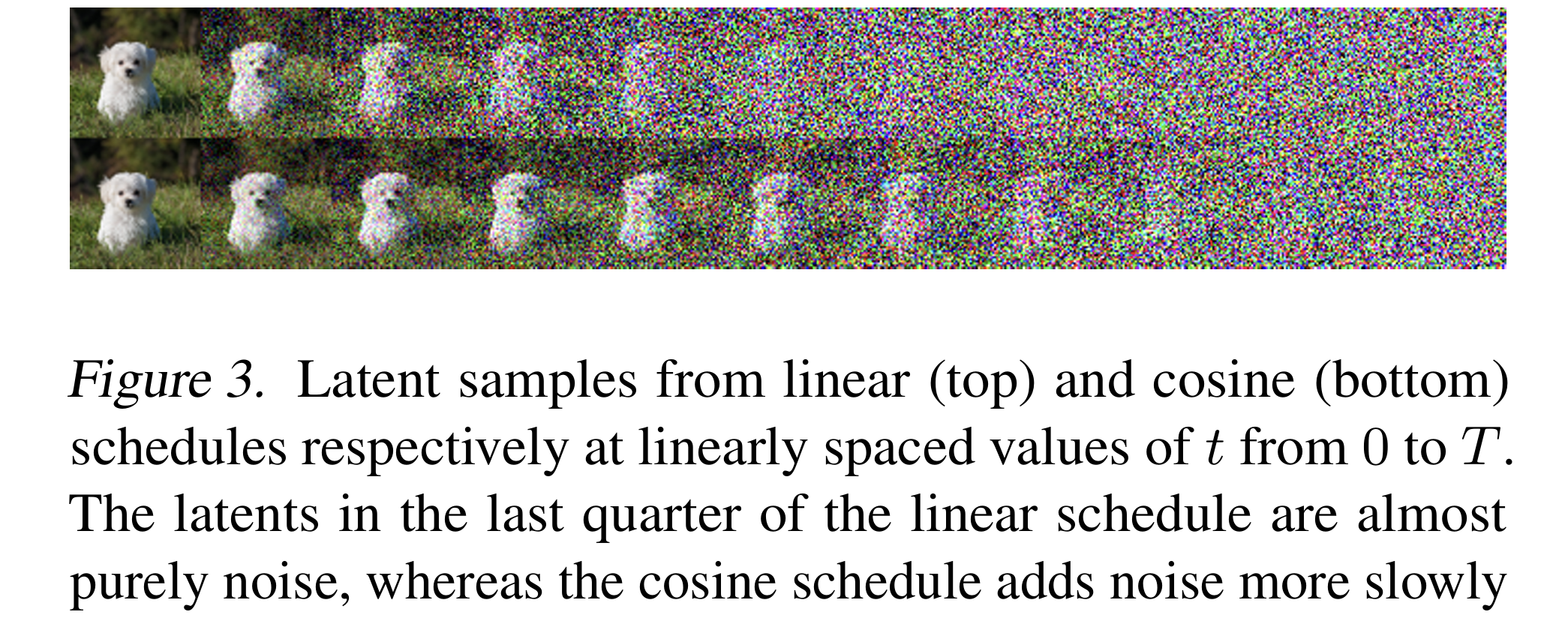
TL;DR: The cosine schedule adds noise more slowly and evenly. As a consequence, the “amount of denoising” is spread more evenly across timesteps. The model sees a wider range of noise levels during training instead of many steps that are already pure noise. Training stability and sample quality » those of a linear schedule.

3. Learned variance in the reverse process

In DDPM, the reverse step is a Gaussian whose mean $\mu_\theta(x_t, t)$ is given by the network (via the predicted noise $\varepsilon_\theta$), and whose variance is fixed to the true posterior variance $\tilde{\beta}_t$:

$$p_\theta(x_{t-1}|x_t) = \mathcal{N}(x_{t-1}; \mu_\theta(x_t,t), \tilde{\beta}_t I)$$

Recall from Part 1 that the true posterior $q(x_{t-1}|x_t, x_0)$ is tractable when conditioned on $x_0$, and is a Gaussian with:

$$\tilde{\mu}_t(x_t, x_0) = \frac{\sqrt{\bar{\alpha}_{t-1}} \cdot \beta_t}{1 - \bar{\alpha}_t} x_0 + \frac{\sqrt{\alpha_t} \cdot (1 - \bar{\alpha}_{t-1})}{1 - \bar{\alpha}_t} x_t$$

$$\tilde{\beta}_t = \frac{1 - \bar{\alpha}_{t-1}}{1 - \bar{\alpha}_t} \beta_t$$

DDPM fixes the reverse-step variance $\tilde{\beta}_t$ and does not learn it.

Improved DDPM instead parameterizes the variance and learns it. Specifically:

• It parameterizes $\Sigma_\theta(x_t, t)$ as a log-domain interpolation between $\beta_t$ and $\tilde{\beta}_t$ - i.e., the upper and lower bounds on the reverse-step variance. The network outputs a vector $v$ (one component per dimension), and the variance$^3$ is:

$$\boxed{\Sigma_\theta(x_t, t) = \exp\bigl(v \log \beta_t + (1 - v) \log \tilde{\beta}_t\bigr)}$$

At first, I took this formulation for granted and just agreed with what the authors proposed here. But after learning more about it, I realized how and why they were able to come up with this:

• $\Sigma_\theta(x_t, t)$ needs to stay within the range $[\tilde{\beta}_t$, $\beta_t]$, which is known to be the reasonable interval for the reverse-step variance. However, this range is very small, making direct prediction unstable.

• Hence, the authors formulated it such that the network predicts an interpolation weight $v$, and maps it to that range via a geometric interpolation in the log-space. When $v \in [0, 1]$, this keeps the output strictly between the two bounds; the VLB loss naturally discourages the network from pushing $v$ outside this range.

Now that we understand how $\Sigma_\theta(x_t, t)$ is formulated, the next question is, how do we train/learn it?

• We need a loss that is sensitive to the specific choice of variance. $L_{simple}$ (the noise-prediction loss) is not, since it only depends on the predicted mean.

• Hence, the VLB is the right signal because it directly measures, at each timestep $t$, how close the model’s reverse step $p_\theta(x_{t-1}|x_t)$ is to the true posterior $q(x_{t-1}|x_t, x_0)$. And this closeness depends on both the mean and variance.

Since both distributions are Gaussian, the KL divergence has a closed form$^4$:

$$ \mathrm{KL}\bigl( q(x_{t-1}\mid x_t,x_0) ,\big|, p_\theta(x_{t-1}\mid x_t) \bigr) = \tfrac{1}{2} \left[ \log \tfrac{\Sigma_\theta(x_t,t)}{\tilde{\beta}_t} + \tfrac{\tilde{\beta}_t + |\tilde{\mu}_t(x_t,x_0) - \mu_\theta(x_t,t)|^2}{\Sigma_\theta(x_t,t)} - 1 \right] $$

The better $\Sigma_\theta$ matches the true posterior’s variance (or spread) at each step, the smaller this KL term and the tighter the VLB.

We’ve talked about the variance, what about the mean? In principle, the same VLB term could also be used to update $\mu_\theta$, but the paper deliberately keeps the two separated:

• a stop-gradient is applied to $\mu_\theta$ inside the VLB term, so gradients from the VLB only flow into $\Sigma_\theta$, which $\mu_\theta$ is trained solely by $L_{simple}$

• this separation is important for stability - more on it in Section 4.

TL;DR: Why do we need to learn the variance instead of keeping it fixed?

• A fixed $\tilde{\beta}_t$ is a one-size-fits-all choice: the same variance is used at every step regardless of what the model actually needs.

• Learned variance lets the model adapt. It can use a smaller variance when it’s confident about the denoising direction, and a larger one when uncertain.

• In general, this tighter fit to the data improves the log-likelihood and in practice often improves sample quality (measured by FID) as well.

4. Hybrid training objective

Recall in this section from Part 1 how DDPM training uses a simple loss:

$$\mathcal{L}_{\text{simple}} = \mathbb{E}[| \varepsilon - \varepsilon_\theta(x_t, t) |^2]$$

which corresponds to predicting the noise, and this loss actually gives good samples even though it’s not the full VLB.

Improved DDPM keeps the simple loss $L_{simple}$ for the mean $\mu_\theta$ (noise prediction), and adds the VLB so that the variance $\Sigma_\theta$ is also trained with the proper variational objective.

The total loss is a hybrid loss:

$$\boxed{\mathcal{L} = \mathcal{L}_{\text{simple}} + \lambda \mathcal{L}_{\text{vlb}}}$$

Here:

• $\mathcal{L}_{\text{vlb}}$ is the negative variational lower bound, so we minimize $\mathcal{L}_{\text{vlb}}$.

• The scalar $\lambda$ is small (e.g., 0.001) so that the main signal still comes from $\mathcal{L}_{simple}$ and training remains stable.

The paper defines $\mathcal{L}_{\text{vlb}}$ explicitly as a sum of per-step terms:

$$\mathcal{L}_{\text{vlb}} = L_0 + L_1 + \cdots + L_{T-1} + L_T$$

where:

$$L_0 = -\log p_\theta(x_0 | x_1)$$

$$L_{t-1} = D_{\text{KL}}\bigl[ q(x_{t-1}|x_t, x_0) | p_\theta(x_{t-1}|x_t)\bigr] \quad \text{for } t = 1, \ldots, T$$

$$L_T = D_{\text{KL}}\bigl[q(x_T|x_0) | p(x_T)\bigr]$$

• $L_0$ is the reconstruction term - how well the model recovers the clean image $x_0$ from $x_1$ (the slightly noised version). It is the only term that directly measures image reconstruction quality.
• $L_{t-1}$ is the denoising term at each step - the KL divergence between the true posterior $q(x_{t-1}|x_t, x_0)$ and the model’s reverse step $p_\theta(x_{t-1}|x_t)$. Since both are Gaussians, this has a closed form (see above). This is the term that provides the training signal for $\Sigma_\theta$.
• $L_T$ is the prior matching term - how close the fully noised $x_T$ is to a standard Gaussian $\mathcal{N}(0, I)$. This does not depend on $\theta$ at all (the forward process is fixed), so it is a constant during training and can be ignored for optimization.

During backprop, gradients from $\mathcal{L}_{\text{vlb}}$ would normally flow through both $\Sigma_\theta$ and $\mu_\theta$, essentially updating both. But the paper applies a stop-gradient to $\mu_\theta$ inside $\mathcal{L}_{\text{vlb}}$, which means: when computing the VLB loss, the network’s mean output $\mu_\theta$ is treated as a fixed constant. Gradients are blocked from flowing through it. So $\mathcal{L}_{\text{vlb}}$ can only update $\Sigma_\theta$.

The reason behind this design choice is actually so interesting:

• Because $\mathcal{L}_{\text{vlb}}$ and $\mathcal{L}_{\text{simple}}$ would otherwise send competing gradient signals to $\mu_\theta$ - the two losses are not perfectly aligned, and letting both update the mean simultaneously destabilizes training.

• The clean separation, then, looks like this: $\mathcal{L}_{\text{simple}}$ is solely responsible for teaching the network to predict noise (training $\mu_\theta$), and $\mathcal{L}_{\text{vlb}}$ is solely responsible for teaching the network what variance to use at each step (training $\Sigma_\theta$).

Section 2: Code

1. Improved DDPM official PyTorch implementation

The codebase for Improved DDPM is made public by the authors at: https://github.com/openai/improved-diffusion

It’s very simple to navigate, so I highly recommend you check it out.

2. My PyTorch implementation

The GitHub repo for my PyTorch implementation of Improved DDPM can be found here: halannhile/improved-ddpm.

If you’ve looked through my DDPM implementation, the files dataset.py, unet.py, noise_scheduler.py and utils.py are unchanged. The main new improvements are in these files: diffusion.py, train.py and sample.py, for which I’ve added a suffix _improved to the file names.

For some reasons, I ran into lots of issues with Improved DDPM (NaN loss, noisy generated samples at 100 epochs, etc.) and had to implement many fixes that I guess the original authors did not have to, probably because they trained with a much bigger and more robust model. I’ve covered some of these fixes in the section below, hope they’re useful for when you run into similar issues in other projects. One valuable lesson I’ve learned throughout my experiences implementing deep learning models is that sometimes they can fail silently without us knowing, which is so much more dangerous and harder to debug than them angrily throwing errors at us.

2.1. The cosine noise schedule:

The cosine schedule is already covered in detail in this section of the DDPM post - I implemented it there since it was a small enough change to drop straight into the existing pipeline.

2.2. Learned variance:

In DDPM, the U-Net outputs C channels (one noise prediction per image channel). In Improved DDPM, it outputs 2*C channels - the first half is the noise prediction $\varepsilon_\theta$, the second half is the raw variance weights $v$.

Splitting the U-Net output:

def _predict(self, x, t):
    out = self.model(x, t)   # [B, 2C, H, W]
    C = out.shape[1] // 2
    return out[:, :C], out[:, C:]  # noise_pred, v

Computing the learned log variance:

The network outputs raw (unconstrained) weights $v$. I pass them through sigmoid to get $\hat{v} \in (0, 1)$, then interpolate in log-space between the two known bounds:

$$\log \Sigma_\theta = \hat{v} \cdot \log \beta_t + (1 - \hat{v}) \cdot \log \tilde{\beta}_t$$

def _learned_log_variance(self, v, t):
    betas = self.noise_scheduler.betas[t][:, None, None, None]
    beta_tilde = self.noise_scheduler.posterior_variance[t][:, None, None, None]

    log_beta = torch.log(betas.clamp(min=1e-20))
    log_beta_tilde = torch.log(beta_tilde.clamp(min=1e-20))

    v = torch.sigmoid(v)  # constrain to (0, 1)
    return v * log_beta + (1 - v) * log_beta_tilde

Note: sigmoid here is not in the original paper - the paper just uses raw $v$. I added it because from my experience training on MNIST for the first time, without it, large $|v|$ at random initialization causes log(beta_tilde_t) (which is very negative for small $t$) to be amplified, exp(log_var) overflows to inf, and the loss is NaN from the very first batch. So I had to retrain MNIST with this small change here.

How the learned variance is used during sampling:

In the reverse loop, instead of using the fixed $\tilde{\beta}_t$ like DDPM does, I compute $\Sigma_\theta$ from the model output:

if i > 0:
    log_var = self._learned_log_variance(v, t)
    sigma = torch.exp(0.5 * log_var)   # sqrt(Sigma_theta)
    noise = torch.randn_like(x)
else:
    sigma = 0.0   # no noise at the final step (t=0 is deterministic)
    noise = torch.zeros_like(x)

x = mean + sigma * noise

2.3. Hybrid loss:

The hybrid loss adds a VLB term on top of the familiar $L_\text{simple}$ from DDPM.

Computing the KL term ($L_\text{vlb}$):

Reminder: Both the true posterior $q(x_{t-1} | x_t, x_0)$ and the model posterior $p_\theta(x_{t-1} | x_t)$ are Gaussians, so the KL divergence has a closed form:

$$L_\text{vlb} = \frac{1}{2} \left[ \log \frac{\Sigma_\theta}{\tilde{\beta}_t} + \frac{\tilde{\beta}_t + (\tilde{\mu}_t - \mu_\theta)^2}{\Sigma_\theta} - 1 \right]$$

The true posterior mean $\tilde{\mu}_t$ is computed from $x_0$ and $x_t$ using the closed-form coefficients from the DDPM paper. The model mean $\mu_\theta$ is computed from the noise prediction using the same reverse formula as DDPM.

The key line is noise_pred.detach() - this is the stop-gradient that prevents $L_\text{vlb}$ from touching the noise prediction. Without it, the KL and MSE losses would send competing signals to $\mu_\theta$ and destabilize training.

def _vlb_terms(self, x_0, x_t, t, noise_pred, log_var):
    # precomputed schedule tensors, shaped [B, 1, 1, 1] for broadcasting
    alpha = self.noise_scheduler.alphas[t][:, None, None, None]
    alpha_cumprod = self.noise_scheduler.alphas_cumprod[t][:, None, None, None]
    alpha_cumprod_prev = self.noise_scheduler.alphas_cumprod_prev[t][:, None, None, None]
    betas = self.noise_scheduler.betas[t][:, None, None, None]
    beta_tilde = self.noise_scheduler.posterior_variance[t][:, None, None, None]

    # true posterior mean: mu_tilde_t = coeff1 * x_0 + coeff2 * x_t
    coeff1 = torch.sqrt(alpha_cumprod_prev) * betas / (1.0 - alpha_cumprod)
    coeff2 = torch.sqrt(alpha) * (1.0 - alpha_cumprod_prev) / (1.0 - alpha_cumprod)
    true_mean = coeff1 * x_0 + coeff2 * x_t
    true_log_var = torch.log(beta_tilde.clamp(min=1e-20))

    # model mean: mu_theta (stop-gradient on noise_pred so L_vlb only trains the variance)
    sqrt_recip_alpha = 1.0 / torch.sqrt(alpha)
    sqrt_one_minus_alpha_cumprod = torch.sqrt(1.0 - alpha_cumprod)
    model_mean = sqrt_recip_alpha * (
        x_t - (betas / sqrt_one_minus_alpha_cumprod) * noise_pred.detach()
    )

    # KL divergence (closed form for two Gaussians)
    diff_sq = (true_mean - model_mean) ** 2
    kl = 0.5 * (
        log_var - true_log_var
        + (torch.exp(true_log_var) + diff_sq) / torch.exp(log_var)
        - 1.0
    )

    kl = kl.mean(dim=[1, 2, 3])   # average over C, H, W -> [B]

    # mask out t=0: beta_tilde_0 = 0, KL is undefined there
    mask = (t > 0).float()
    return kl * mask

Putting it together in training_losses():

def training_losses(self, x_0):
    t = self.noise_scheduler.sample_timesteps(batch_size)
    noise = torch.randn_like(x_0)
    x_t = self.noise_scheduler.add_noise(x_0, t, noise)

    noise_pred, v = self._predict(x_t, t)

    # L_simple: trains the noise prediction (identical to DDPM)
    l_simple = F.mse_loss(noise_pred, noise)

    # L_vlb: trains the variance (stop-gradient on noise_pred inside)
    log_var = self._learned_log_variance(v, t)
    l_vlb = self._vlb_terms(x_0, x_t, t, noise_pred, log_var).mean()

    return l_simple + self.lambda_vlb * l_vlb

2.4. Miscellaneous

As aforementioned, these are the fixes I had to implement for my model.

Gradient clipping (train_improved.py): the VLB term can produce large gradient spikes early in training when the variance head outputs large random values. Clipping the gradient norm to 1.0 before each optimizer step prevents these from destabilizing the noise prediction:

optimizer.zero_grad()
loss.backward()
torch.nn.utils.clip_grad_norm_(ddpm.model.parameters(), max_norm=1.0)
optimizer.step()

Cosine LR scheduler (train_improved.py): unlike the original DDPM which uses a fixed learning rate, I add a cosine annealing scheduler that decays the LR from its initial value to $10^{-6}$ over training. This helps the model keep improving in later epochs instead of bouncing around a plateau:

scheduler = torch.optim.lr_scheduler.CosineAnnealingLR(optimizer, T_max=args.epochs, eta_min=1e-6)
# ... inside the epoch loop:
scheduler.step()

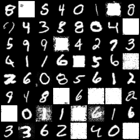
Clamping during sampling (diffusion_improved.py): occasionally, a few samples diverge during the reverse process - the learned variance at some step is large, pushing x far outside the valid range, and it never recovers. Clamping x to [-2, 2] after each reverse step prevents this. I use [-2, 2] rather than [-1, 1] because intermediate $x_t$ values can legitimately exceed [-1, 1] during denoising:

x = (mean + sigma * noise).clamp(-2, 2)

The final clamp(-1, 1) and denormalization back to [0, 1] happens at the very end of sample(), after the loop. The original authors did not need this because their larger, more thoroughly trained model produces well-behaved variance predictions throughout sampling. With a smaller model trained for fewer steps, like mine, the variance head occasionally misfires at some timestep, and clamping acts as a guard rail to catch those rare instances.

This is how I found out about this issue, by observing the generated samples grid at epoch 300:

Thanks to Claude Code for helping me debug and think of a fix. I find it helpful to engage AI agents during the debugging process, since they sometimes suggest really good solutions that I was not aware of at all. Apart from this, it’s necessary that you try to write the code yourself to solidify your understanding.

Section 3: Results from the trained model

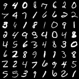
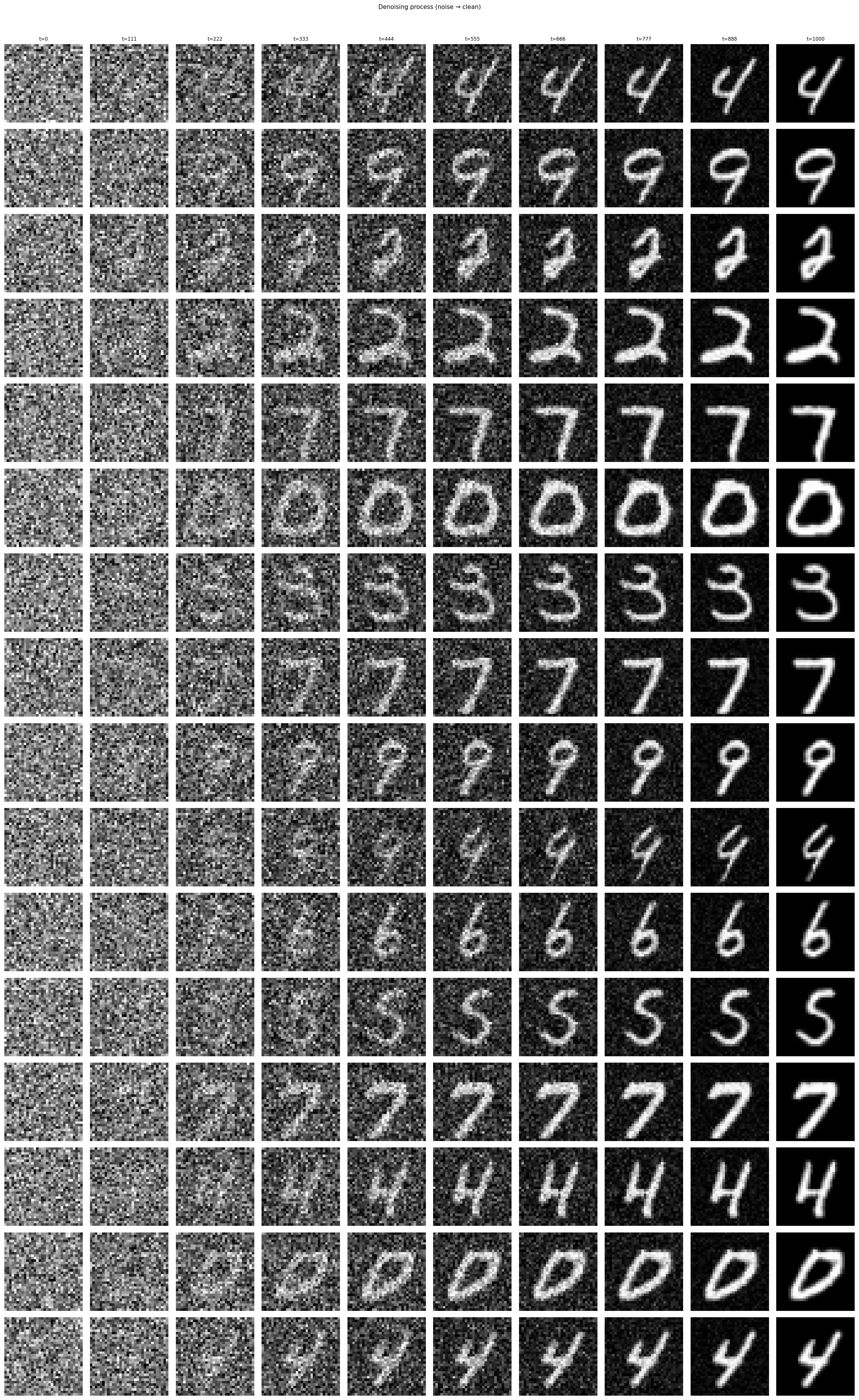
I trained on MNIST for 300 epochs. These are the generated samples and visualizations of the denoising process:

Section 4: Recap & what’s next

Next, I’m looking forward to diving into the paper Denoising Diffusion Implicit Models (DDIM) (Song et al., 2021), which dramatically speeds up sampling from 1000 steps to as few as 50.

Diffusion models are not easy to grasp and implement, if I’m being honest. But once you overcome the initial frustration and overwhelm, it’s a very rewarding learning experience.

Useful Resources

Theory

• Lil’Log - What are diffusion models?
• Jia-Bin Huang - How I Understand Diffusion Models

Code

• Official Improved DDPM repo written in PyTorch

Citation

Le, Nhi. "Diffusion Models - Part 2: Improved DDPM". halannhile.github.io (March 2026). https://halannhile.github.io/posts/improved-ddpm/

BibTeX:

@article{nhi2025ddpm,
  title = {Diffusion Models - Part 2: Improved DDPM},
  author = {Nhi},
  journal = {halannhile.github.io},
  year = {2026},
  month = {March},
  url = "https://halannhile.github.io/posts/improved-ddpm/"
}