One of the places my curiosity took me to recently is Diffusion Models. Let’s start with Denoising Diffusion Probabilistic Models (DDPM; Ho et al. 2020).
The GitHub repo for my PyTorch implementation of DDPM with instructions on how to train and generate images can be found here: halannhile/ddpm.
Table of Contents
- Overview of DDPM
- The forward process
- The reverse process
- The training objective
- Training & sampling algorithms
Section 3: Recap & What’s Next
Section 1: Theory
1. Overview of DDPM
Prior to diffusion models, GANs largely dominated the conversation around high-fidelity image generation. Diffusion models, made practical and popular by DDPM, changed that narrative and have since become the dominant paradigm in modern image generation.
The core idea behind diffusion models is surprisingly elegant: train a neural network to gradually denoise an image corrupted with (Gaussian) noise.
In other words, if we gradually destroy an image by adding noise over hundreds or thousands of steps until it becomes pure noise - and we train a model to gradually undo that process - we end up with a model that can generate images from scratch, starting from random noise. Diffusion models typically use Gaussian noise because it makes the forward and reverse processes mathematically tractable, and the training stable. Gaussian distribution, albeit simple, in certain cases offers nice properties that make hard problems manageable.
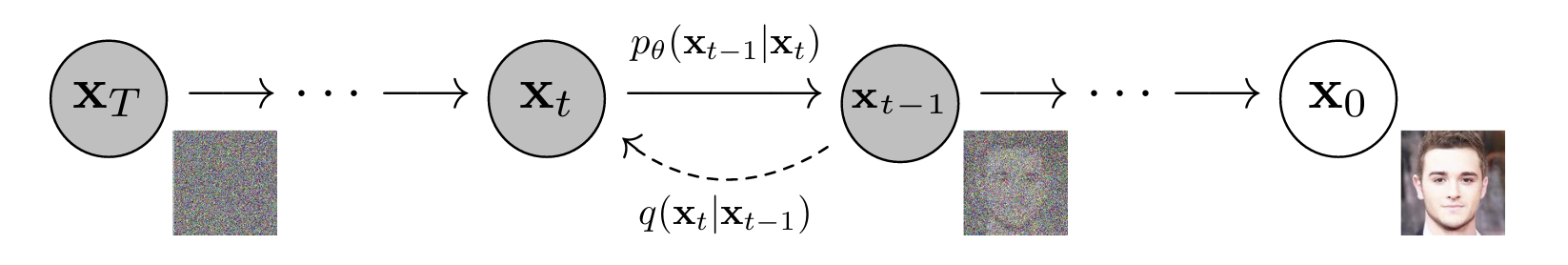
The two processes of DDPM
DDPM is built on two complementary processes:
1. Forward process (also called the forward diffusion process): starting with a clean image $x_0$, we systematically corrupt it over $T$ timesetps by adding small amounts of Gaussian noise. At the end of the diffusion process, the image becomes pure Gaussian noise $\mathcal{N}(0, I)$.
2. Reverse process (also called the reverse diffusion process): we start from pure noise and learn to denoise step-by-step until a clean image emerges. This is what the core architecture, the U-Net neural networks, learns to do.
At generation time, we sample random noisy image $x_T \sim \mathcal{N}(0, I)$ and run the reverse process to produce a new, clean image.
2. The forward process
2.1. The original form
At each time step $t$, a small amount of Gaussian noise is added to the previous image $x_{t-1}$ to give us a slighly more noisy image $x_{t}$. The amount of noise is controlled by a variance scheduler $\beta_{t}$ where $0 < \beta_t < 1$. In practice the schedule is usually increasing: $0 < \beta_1 < \beta_2 < … < \beta_T < 1$.
$$q(x_t | x_{t-1}) = \mathcal{N}(x_t; \sqrt{1 - \beta_t}\ x_{t-1}, \beta_t I)$$
In other words: to get $x_t$, we scale down $x_{t-1}$ slightly by $\sqrt{1 - \beta_t}$ and add noise with variance $\beta_t$.
2.2. The closed-form shortcut & reparameterization trick
Running the forward process step-by-step to get from $x_0$ to $x_t$ is painfully slow, since we need to generate all the intermediate steps sequentially $x_{1}, x_{2}, …, x_{t-1}$. Fortunately, the math works out so that we can jump directly from $x_0$ to any $x_t$ in a single step. I found this to be incredibly beautiful and elegant.
The full derivation is not included here for brevity. Please refer to my list of useful resources for more details.
Define:
$$\alpha_t = 1 - \beta_t$$
$$\bar{\alpha}_t = \prod_{s=1}^{t} \alpha_s$$
which is the cumulative product of all $\alpha$ values up to timestep $t$.
Then the closed-form forward process is:
$$q(x_t|x_0) = \mathcal{N}(x_t; \sqrt{\bar{\alpha}_t}x_0, (1-\bar{\alpha}_t)I)$$
which we can sample using the reparameterization trick as:
$$\boxed{x_t = \sqrt{\bar{\alpha}_t} x_0 + \sqrt{1 - \bar{\alpha}_t} \varepsilon, \quad \varepsilon \sim \mathcal{N}(0, I)} \quad (4)$$
This is Equation 4 from the paper, and in my opinion it’s the single most important formula for implementing DDPM. It means:
- When $t$ is small: $\bar{\alpha}_t \approx 1$, so $x_t \approx x_0$ (barely noisy)
- When $t$ is large: $\bar{\alpha}_t \approx 0$, so $x_t \approx \varepsilon$ (pure noise)
This can be understood intuitively as follows:
In $(4)$, $\sqrt{\bar{\alpha}_t} x_0$ is the signal and $\sqrt{1 - \bar{\alpha}_t} \varepsilon$ is the error. The two coefficients always satisfy:
$$\bar{\alpha}_t + (1 - \bar{\alpha}_t) = 1$$
meaning signal and noise always sums to 1 in variance. As $t$ increases and $\bar{\alpha}_t$ decreases towards zero: the signal shrinks (the original image fades away) and the noise grows (Gaussian noise takes over). At $t = T$, $x_t \approx \epsilon \sim \mathcal{N}(0, 1)$, i.e., the image has been corrupted completely.
What exactly is the reparameterization trick?
I exclude most mathematical derivations from this blog but since Equation (4) is so important in DDPM, I want to explain more about the reparameterization trick in Gaussian distribution. Let’s first understand its basic statistical derivation.
Say we have a random variable sampled from a distribution whose parameters (mean & variance) we want to optimize:
$$x \sim \mathcal{N}(\mu, \sigma^2)$$
If we want to compute gradients wrt. $\mu$ and $\sigma$, we have a problem: we can’t propagate through a sampling operation. Sampling is stochastic - it’s not a deterministic function we can differentiate through. The gradient of “randomly draw a number” wrt. the distribution’s parameters is undefined.
The trick works by separating the stochasticity from the parameters: Instead of sampling $x \sim \mathcal{N}(\mu, \sigma^2)$ directly, we do:
$$\epsilon \sim \mathcal{N}(0, 1)$$
which is error sampled from a fixed, parameter-free distribution. Then:
$$x = \mu + \sigma \cdot \epsilon$$
This produces exactly the same distribution over $x$. But now the randomness is isolated in $\epsilon$, which has no parameters to differentiate through. The computations we need to perform flow cleanly through $\mu$ and $\sigma$ because the transformation $x = \mu + \sigma \cdot \epsilon$ is just arithmetic and fully differentiable.
We’ve turned from “sampling from a parameterized distribution”, to “sampling from a standard Gaussian $\mathcal{N}(0,1)$, then scale by $\sigma$ and shift by $\mu$”.
In fact, the reparameterization trick, together with a key property of Gaussian distribution that the sum of two independent Gaussians is also Gaussian helps us iteratively derive $x_1$ from $x_0$, substitute into the derivation of $x_2$ from $x_1$ to get $x_0$ from $x_2$, so on and so forth, until we get to the final form in $(4)$.
The parameterization trick also means $(4)$ can be understood as follows: to get from $x_t$ from $x_0$ is simply a shift-and-scale of an independent noise $\epsilon$.
Why this trick matters for DDPM:
Without it, for each training sample, we’d need to run $t$ sequential forward steps just to create the noisy input, and $t$ is randomly sampled up to $T$ each time (in DDPM, $T = 1000$). With the closed-form expression, creating $x_t$ from $x_0$ takes exactly one operation regardless of how large $t$ is.
3. The reverse process
The reverse process learns how to undo all the corruptions we’ve made to the clean input images during the forward process.
What GANs attempt to do is to go from 100% noise to 0% noise in one shot, essentially asking the model to hallucinate an entire image from scratch with no intermediate guidance - this is notoriously unstable to train.
With DDPM, we ask: given a noisy image $x_t$, what does the slightly less noisy version $x_{t-1}$ look like? If we could answer this for every $t$, we could start from pure noise $x_T$ and walk all the way back to a clean image $x_0$ in incremental steps. Taking many small steps rather than one giant leap is the exact same reason why the forward process adds noise gradually: small steps are predictable, large steps aren’t.
In fact, each denoising step is responsible for undoing roughly $1/T$ of the total noise. Because of this manageable and tractable denoising process, DDPM generates higher-quality images than GANs.
3.1. The intractable distribution of $x_{t-1}$
Unfortunately, the true reverse distribution $q(x_{t-1}|x_t)$ is intractable, since it requires knowing the true distribution of input images $p(x_0)$, which is the very thing we’re trying to learn.
3.2. The tractable distribution of $x_{t-1}$
Fortunately, the conditional reverse distribution $q(x_{t-1}|x_t, x_0)$ - i.e., where we’re given not only $x_t$ but also the original clean image $x_0$, is tractable. It’s just a Gaussian:
$$q(x_{t-1} | x_t, x_0) = \mathcal{N}(x_{t-1}; \tilde{\mu}_t(x_t, x_0), \tilde{\beta}_t I)$$
where the posterior mean is:
$$\tilde{\mu}_t(x_t, x_0) = \frac{\sqrt{\bar{\alpha}_{t-1}}\cdot \beta_t}{1 - \bar{\alpha}_t} x_0 + \frac{\sqrt{\alpha_t} \cdot (1 - \bar{\alpha}_{t-1})}{1 - \bar{\alpha}_t} x_t$$
and the posterior variance is:
$$\tilde{\beta}_t = \frac{1 - \bar{\alpha}_{t-1}}{1 - \bar{\alpha}_t} \beta_t$$
The math seems to come out of nowhere. But intuitively, the posterior mean is a weighted combination of 2 things:
- a contribution from the original image $x_0$
- a contribution from the current noisy image $x_t$
Only one caveat: we don’t know $x_0$ at inference/generation time! But that’s the whole point of training a neural nets, so that we can predict $x_0$. During training, we have access to $x_0$ and hence the model can be supervised trained here. During inference, the model substitutes with its own prediction $\hat{x}_0$.
In fact, in the above formula:
the true posterior mean $\tilde{\mu}_t(x_t, x_0)$ is intractable because it depends on $x_0$ which we don’t have at inference
the true posterior variance $\tilde{\beta}_t$ is fully tractable since it depends only on 3 values , which are all fixed, precomputed constants from the noise schedule that require no neural network and no knowledge of $x_0$.
3.3. What the neural network learns: noise prediction (instead of clean image prediction)
The DDPM paper makes an interesting design choice: rather than training the model to predict $x_0$ directly, it’s trained to predict the noise that was added to $x_0$ to create $x_t$. We can then “subtract” this predicted noise to get $\hat{x}_0$ (this is not a simple subtraction but has some scaling factor).
This trained model is $\epsilon_{\theta}(x_t, t)$.
Why? I asked myself the same question. Below are some motivating factors:
- predicting Gaussian noise in the same range $\mathcal{N}(0,1)$ is easier than predicting a full clean image from noisy input.
- at large timesteps where the image is noisy, asking the model “what was the original clean image?” is nearly impossible since there’s little signal left. But asking “what Gaussian noise was added?” is more tractable since there’s at least still some structure from Gaussian noise that we can partially infer.
- one neat thing is: predicting noise leads to a simple MSE loss (read more below).
3.4. What does one denoising step look like?
Once noise $\epsilon_{\theta}(x_t, t)$ is predicted, we can predict $\hat{x}_0$ via:
$$\hat{x}_0 = \frac{x_t - \sqrt{1 - \bar{\alpha}_t} \cdot \varepsilon_\theta(x_t, t)}{\sqrt{\bar{\alpha}_t}}$$
We then plug this into the posterior mean $\mu_\theta(x_t,t)$ and simplify to get the sampling update:
$$\boxed{\mu_\theta(x_t, t) = \frac{1}{\sqrt{\alpha_t}} \left( x_t - \frac{\beta_t}{\sqrt{1 - \bar{\alpha}_t}} \cdot \varepsilon_\theta(x_t, t) \right)}$$
In words, one denoising step works like this:
take the current noisy image $x_t$, subtract out the predicted noise $\varepsilon_\theta(x_t, t)$ (scaled appropriately), and rescale, gives us the mean $\mu_\theta$ of the reverse distribution $p_\theta(x_{t_1}|x_t)$
to actually sample $x_{t-1}$, we then draw from a Gaussian distribution at that mean:
$$\boxed{x_{t-1} = \mu_\theta(x_t, t) + \sqrt{\tilde{\beta}_t} z, \quad z \sim \mathcal{N}(0,1)}$$
A very important note here is: after computing the mean $\mu_\theta$, we don’t use it directly as $x_{t-1}$. Instead, we’re adding back a small amount of fresh Gaussian noise, i.e., scaled noise $\sqrt{\tilde{\beta}_t} z$.
Why do we add noise back during sampling?
This felt counterintuitive to me at first. We’re trying to denoise, why add more? The reason is diversity, without which the model isn’t truly generative.
If every reverse step were fully deterministic, then every starting noise $x_T$ would map to the same final image. The stochasticity at each step, via the added scaled noise, means that the reverse trajectories can diverge, allowing the model to generate diverse images.
The one exception is the final step ($t=1 \rightarrow t=0$) where we set $z=0$ and use the mean directly as the sampled image. At this point, adding noise would add random variation to the nearly-finished image, which would corrupt the fine details rather than add useful diversity. Hence, the last step is fully deterministic.
4. The training objective
In many blogs and videos that deep-dive into DDPM, the authors discuss this concept of the ELBO (Evidence Lower Bound), which involves a sum of KL divergences at each step. (Simply put, KL divergence is a measurement of how different one distribution is from another).
The math behind the ELBO can be terrifying to beginners. But luckily for us, the DDPM authors provide one key finding that the training objective can be simplified dramatically into a simple MSE loss:
$$\boxed{L_\text{simple} = \mathbb{E}_{t, x_0, \varepsilon} \left[ | \varepsilon - \varepsilon_\theta(\sqrt{\bar{\alpha}_t} x_0 + \sqrt{1-\bar{\alpha}_t} \varepsilon, t) |^2 \right]}$$
This is Equation 14 in the paper. In simple words, the training objective says that we:
- sample a random timestep
- add noise to the image
- ask the model what noise was added
- minimize the MSE between the true noise and the prediction
5. Training & sampling algorithms
My PyTorch implementation of DDPM is built around these 2 algorithms from the paper:
Algorithm 1: Training
repeat:
    x_0 ~ q(x_0)                              # sample a real image
    t ~ Uniform({1, ..., T})                  # sample a random timestep
    ε ~ 𝒩(0, I)                               # sample noise

    x_t = √ᾱ_t · x_0 + √(1-ᾱ_t) · ε         # corrupt image (closed-form forward)

    Take gradient step on:
        ∇_θ ‖ε - ε_θ(x_t, t)‖²               # MSE between true and predicted noise
until converged
Algorith2 : Sampling (Reverse Diffusion)
x_T ~ 𝒩(0, I)                                                     # start from pure noise
for t = T, T-1, ..., 1:
    z ~ 𝒩(0, I) if t > 1, else z = 0                              # no noise at final step
    x_{t-1} = (1/√α_t)(x_t - β_t/√(1-ᾱ_t) · ε_θ(x_t,t)) + √β̃_t·z   # denoise one step
end for
return x_0                                                          # generated image
Section 2: Code
You can find my PyTorch implementation here.
I referenced many different PyTorch implementations of DDPM (you can find them in my list of useful resources) and I wrote my own version in the end. All docstrings & comments are my own.
Here’s how my repo is organized:
.
├── noise_scheduler.py   # precomputes β, α, ᾱ schedules; implements forward process
├── unet.py              # U-Net model: ε_θ(x_t, t)
├── diffusion.py         # DDPM class: training_losses() and sample()
├── dataset.py           # dataLoaders (for MNIST and CIFAR-10)
├── utils.py             # EMA (exponential moving average), checkpointing
├── train.py             # main training loop
└── sample.py            # inference: load checkpoint & generate images
Here’s the dependency graph:
train.py / sample.py
       ├── diffusion.py
       │       ├── noise_scheduler.py
       │       └── unet.py
       ├── dataset.py
       └── utils.py
Since I’ve included detailed docstrings and comments to my code, in the following sections, I will only explain key sections of the code that implement very interesting techniques.
1. The noise scheduler: noise_scheduler.py
1.1. Precomputing terms
The NoiseScheduler class is responsible for a major task in the forward process: precomputing all the constants from the paper so they can be looked up constantly during training, rather than recomputed at each step.
Specifically, the noise scheduler precomputes $\beta_t, \alpha_t, \bar{\alpha}_t$ and other terms that include $\bar{\alpha}_t$, and also implements Eq. 4
# create beta schedule
if schedule_type == 'linear':
    self.betas = torch.linspace(beta_start, beta_end, num_timesteps, device=device)
elif schedule_type == 'cosine':
    self.betas = self._cosine_beta_schedule(num_timesteps).to(device)
else:
    raise ValueError(f"Unknown beta schedule type")


# precompute all alphas term in DDPM
self.alphas = 1.0 - self.betas
self.alphas_cumprod = torch.cumprod(self.alphas, dim=0)
self.alphas_cumprod_prev = torch.cat([torch.ones(1, device=device), self.alphas_cumprod[:-1]]) # prepend 1.0 because at t=0, no noise has been added yet

# forward diffusion: q(x_t | x_0) (Eq.9 pg.3)
self.sqrt_alphas_cumprod = torch.sqrt(self.alphas_cumprod)
self.sqrt_one_minus_alphas_cumprod = torch.sqrt(1.0 - self.alphas_cumprod)

# reverse process: q(x_{t-1} | x_t, x_0) (Eq.10 pg.3)
self.sqrt_recip_alphas = torch.sqrt(1.0 / self.alphas)

# posterior variance for sampling (Eq.7 pg.3)
self.posterior_variance = self.betas * (1.0 - self.alphas_cumprod_prev) / (1.0 - self.alphas_cumprod)
Note: all these constants are tensors of shape [T] (one value per timestep) and they never change after initialization.
1.2. The add_noise() method (forward process)
Here, we implement the closed-form formula of Equation 4: $x_t = \sqrt{\bar{\alpha}_t} x_0 + \sqrt{1-\bar{\alpha}_t} \varepsilon$
# create random Gaussian noise epsilon ~ N(0,1) with the same shape as x_0
if noise is None:
    noise = torch.randn_like(x_0)

# lookup coefficients precompted in __init__
sqrt_alpha_prod = self.sqrt_alphas_cumprod[t]
sqrt_one_minus_alpha_prod = self.sqrt_one_minus_alphas_cumprod[t]

# reshape for broadcasting: [B] -> [B,1,1,1], for multiplying with [B, C, H, W]
sqrt_alpha_prod = sqrt_alpha_prod.view(-1, 1, 1, 1) # before: [B], after: [B,1,1,1]
sqrt_one_minus_alpha_prod = sqrt_one_minus_alpha_prod.view(-1, 1, 1, 1)

# x_0.shape = [B, C, H, W]

# x_t = sqrt(alpha_cumprod_t) * x_0 + sqrt(1 - alpha_cumprod_t) * noise
return sqrt_alpha_prod * x_0 + sqrt_one_minus_alpha_prod * noise
Note:
- Broadcasting is an interesting technique in PyTorch, and
.view(-1, 1, 1, 1)is a common pattern where we need to broadcast a scalar for B (batch) across the image’s C (channel), H (height) and W (width) dimension. - Essentially:
[B] → [B, 1, 1, 1]so we can later multiply with[B, C, H, W]
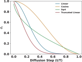
1.3. The cosine $\beta$ schedule
Here I did something different from the original DDPM paper. I implemented an idea from the Improved DDPM paper (Nichol & Dhariwal, 2021), which is to create a cosine schedule for $\beta$.
In fact, the Improved DDPM paper proposes several other interesting improvements to DDPM, besides the cosine $\beta$ schedule, which I might explain in another blog post.
The linear schedule has a known weakness. Because betas increase linearly, the signal-to-noise ratio drops very steeply early on, e.g., by around $t=500$, the image is already almost completely destroyed, so we spend the latter half of the training loop (from $t=501$ to $t=T=1000$) learning to denoise images that are highly corrupted with barely any signal left to recover. This contributes little to learning.
The cosine schedule from the Improved DDPM paper fixes this with a smoother curve, essentially spreading the denoising work more evenly across $T$ timesteps, giving every timestep roughly the same amount of meaningful denoising to work with.
$$\bar{\alpha}_t = \frac{f(t)}{f(0)}, \quad f(t) = \cos\left(\frac{t/T + s}{1 + s} \cdot \frac{\pi}{2}\right)^2$$
Here, $s=0.008$ by default is the small offset to prevent $\beta_t$ from getting too small near $t=0$, which would cause numerical issues.
At the end, $\beta$’s are derived from the ratios of consecutive $\bar{\alpha}$ values and clipped to $[0.0001, 0.0=9999]$ avoid instability near $t = T$.
steps = timesteps + 1 # create T+1 points (0, 1, 2, ..., T) to compute differences later
x = torch.linspace(0, timesteps, steps) # create array [0,1,2,...,T] these are the time indices
alphas_cumprod = torch.cos(
    ((x / timesteps) + s) / (1 + s) * torch.pi * 0.5
) # this is f(t)
alphas_cumprod = alphas_cumprod / alphas_cumprod[0] # = f(t) / f(0) in Eq.17
betas = 1 - (alphas_cumprod[1:] / alphas_cumprod[:-1])

# clip betas to be < 0.9999 to prevent singularities at the end of the diffusion process near t=T
return torch.clip(betas, 0.0001, 0.9999)
2. The U-Net: unet.py
2.1. Architecture
The U-Net is the neural network $\varepsilon_\theta(x_t, t)$ in DDPM. Given a noisy image and a timestep, it outputs a prediction of the noise that was added. This is the only learned component, everything else is basically just deterministic math.
The U-Net has a downsampling stack, and an upsampling stack, with shortcut connections.
You’ll notice that I bolded the phrase “in DDPM” above. This is because there are in fact 2 common backbone architectures for diffusion models:
U-Net: which DDPM used. It has skip connections and attention only at the bottleneck. This was the standard architecture for diffusion models for many years.
Transformer: DiT (Diffusion Transformers) (Peebles & Xie, 2022) was the first paper that made the serious case for replacing U-Net with a Vision Transformer. DiT is now the dominant architecture that pretty much displaced U-Net. Stable Diffusion 3, Flux, Sora, and most modern production systems all use transformer-based backbones. I will have a deep-dive blog into DiT later!
Below is the U-Net architecture I actually implemented:
x_t [B, 3, 32, 32] ──conv0──▶ [B, 64, 32, 32]
                                        │
              ┌─── down1 ──▶ [B, 64, 16, 16]  ←── skip1
              │     down2 ──▶ [B, 128, 8, 8]  ←── skip2
              │     down3 ──▶ [B, 128, 4, 4]  ←── skip3
              │                        │
              │    Bottleneck: bot1 → attn → bot2 → bot3
              │                [B, 128, 4, 4]
              │                        │
              └─── up1(cat skip3) ──▶ [B, 128, 8, 8]
                   up2(cat skip2) ──▶ [B, 64, 16, 16]
                   up3(cat skip1) ──▶ [B, 64, 32, 32]
                                        │
                           outc ──▶ [B, 3, 32, 32] = ε̂
The encoder downsamples three times (32→16→8→4), the bottleneck applies self-attention at 4×4, and the decoder upsamples back to 32×32, concatenating the saved encoder features at each scale.
A quick note on the channel counts:
- The textbook U-Net follows a strictly symmetric pattern where channels double at every encoder stage and halve at every decoder stage, e.g.,
64→128→256down and256→128→64back up. - My implementation doesn’t follow that exactly. The encoder goes
64→64→128→128and the decoder mirrors that with128→128→64→64. The heavy lifting is instead concentrated in the bottleneck, which expands to 256 channels. I was inspired to make this deliberate choice by referencing many DDPM implementations. This architecture keeps the encoder and decoder lean while giving the model maximum capacity at the lowest resolution where the most abstract reasoning happens.
2.2. Sinusoidal embeddings for timesteps
The timestep encodes how noisy the image is, and the network needs to know this information to calibrate its denoising. Hence, we need to encode the timestep into a vector embedding and inject this into every block of the U-Net.
Here, we use a technique invented by the original Transformer paper, Attention Is All You Neeed (Vaswani et al., 2017): sinusoidal position embeeding. In that paper, the authors needed a way to tell the model the position of each token in a sequence, since unlike RNNs, Transformers process all tokens in parallel and have no inherent sense of order. Their solution was to encode each position as a vector of sinusoids at different frequencies, which the DDPM paper directly borrows for encoding timesteps.
'''
How it works:
    For a timestep t and embedding dimension d:
    - Half the dimensions use sin(t / 10000^(2i/d))
    - Other half uses cos(t / 10000^(2i/d))
    where i: the dimension index
'''

class SinusoidalPositionEmbeddings(nn.Module):

    def forward(self, time):
        device = time.device

        half_dim = self.dim // 2

        # create frequency terms: 1/10000^(2i/d)
        embeddings = math.log(10000) / (half_dim - 1)
        embeddings = torch.exp(torch.arange(half_dim, device=device), * -embeddings)

        # ===== MULTIPLY TIMESTEPS BY FREQUENCIES =====
        # Broadcasting: [B, 1] * [1, half_dim] = [B, half_dim]
        embeddings = time[:, None] * embeddings[None, :]

        # ===== APPLY SIN AND COS =====
        # First half_dim dimensions get sin(), second half get cos()
        # Concatenate along last dimension: [B, half_dim] + [B, half_dim] = [B, dim]
        # This creates the full sinusoidal embedding
        # Similar timesteps -> similar embeddings (smooth, continuous encoding)
        embeddings = torch.cat((embeddings.sin(), embeddings.cos()), dim=-1)

        return embeddings # Shape: [B, dim]
Why don’t we use the raw timestep integers?
This is a question I asked myself immediately. Why do through all the trouble of implementing sinusoidal embeddings?
A single scalar is too small to condition a large network. The U-Net has millions of parameters across many layers, and we want the timestep to influence all of them. A single scalar gets added somewhere and then has to propagate its influence through many layers of transformations. By the time it reaches deeper layers, the signal has largely washed out. What we really want is for every layer to have a rich and direct representation of the timestep to condition on. A high-dimensional vector gives each layer far more to work with.
Raw integers don’t encode relationships between timesteps. To a neural network, the integer $t=500$ has no inherent relationship to $t=501$. The model would have to learn from scratch that $t=500$ and $t=501$ are nearby timesteps and require almost identical denoising behavior, which is an inefficient use of training. What we want is a representation where similar timesteps automatically produce similar vectors, so the model can generalize smoothly across the noise schedule. Simply normalizing $t$ to a range like $[0, 1]$ would help with smoothness but still leaves us with a single scalar (same problem we discussed above)
Sinusoidal embeddings solve both problems at once. Without going into technical details of the actual formulae and implementation, we can observe that sinusoidal vector embeedings have some nice properties:
- uniqueness - each timestep maps to a distinct vector, so the model can distinguish them
- smoothness - nearby timesteps produce similar embeddings, so the model naturally generalizes: if it learns to denoise at $t=100$ it already has a good prior for $t=101$
- parameter-free - it’s a fixed deterministic function, no weights needed, unlike a learned embedding table
MLP projection & injecting time vector into every block
We don’t stop after computing the sinusoidal time embeddings. There are 2 more steps wrt. to the timesteps:
Step 1. After the sinusoidal embedding, we have a vector of shape [B, model_channels] (e.g. [B, 64]). This gets projected up to a larger time_emb_dim-dimensional vector (e.g. [B, 256]) via a linear layer and ReLU. Why? Linear helps the network learn how to interpret the timestep, and ReLU adds non-linearity to produce a richer representation of $t$ that the rest of the network can use. This [B, time_emb_dim] vector is computed once per forward pass and shared across all blocks.
self.time_mlp = nn.Sequential(
    SinusoidalPositionEmbeddings(model_channels), # t -> sinusoidal
    nn.Linear(model_channels, time_emb_dim), # project to 256
    nn.ReLU()
)
Step 2. Broadcasting & injecting into every single block in the network: Explaining this would make the blog too lengthy, but to keep it simple:
Broadcasting from
[B, time_emb_dim]to[B, out_ch, 1, 1]is so that the time signal shifts the activations of every feature map channel up or down by a learned amount, giving the convolutions in that block a way to behave differently depending on $t$.The injection happens inside every single block in the U-Net: all three encoder blocks, all three decoder blocks, and each has its own independent linear projection from 256 to its specific channel count. This means the timestep isn’t just a one-time input - it continuously re-conditions the network at every resolution and every depth. So, even though the network weights are identical, the same noisy image passed through the network at $t=100$ vs $t=800$ will produce completely different internal activations and therefore a completely different noise prediction.
2.3. Blocks: Encoder and Decoder
Each Block handles either downsampling (encoder, up=False) or upsampling (decoder, up=True):
class Block(nn.Module):
    ...
    # project time embedding to match output channels
    self.time_mlp = nn.Linear(time_emb_dim, out_ch)

    # UPSAMPLING BLOCK (DECODER)
    if up:
        # Input has 2*in_ch because of skip connections
        self.conv1 = nn.Conv2d(2*in_ch, out_ch, 3, padding=1)
        # ConvTransposed2d upsamples: H,W -> 2H, 2W
        self.transform = nn.ConvTranspose2d(out_ch, out_ch, 4, 2, 1)

    # DOWNSAMPLING BLOCK (ENCODER)
    else:
        self.conv1 = nn.Conv2d(in_ch, out_ch, 3, padding=1)
        # Strided conv downsamples: H,W -> H/2, W/2
        self.transform = nn.Conv2d(out_ch, out_ch, 4, 2, 1)

    # Second convolution
    self.conv2 = nn.Conv2d(out_ch, out_ch, 3, padding=1)

    # Group Normalization (8 groups)
    self.bnorm1 = nn.GroupNorm(8, out_ch)
    self.bnorm2 = nn.GroupNorm(8, out_ch)

    self.relu = nn.ReLU()
Group normalization is used here (instead of batch normalization) because it’s more stable with small batch sizes and doesn’t depend on batch statistics - overall, just works well with diffusion models.
2.4. Bottleneck self-attention
At the lowest resolution (4×4 for 32×32 input), a self-attention layer is applied. Attention is only applied here, at the bottleneck, because attention’s cost scales as $O((H \cdot W)^2)$. At 4×4 (16 tokens), this is cheap. At 32×32 (1024 tokens), it would be very expensive.
Attention is useful in CNNs because they let every spatial position attend to every other position, helping the model maintain a global coherence across the whole image. Traditional CNNs have limited receptive field and can only “see” nearby pixels.
# Inside SimpleAttention.forward():
x = x.view(-1, C, H*W).swapaxes(1, 2)   # [B, C, H, W] → [B, H*W, C]  (treat as tokens)
x_ln = self.ln(x)
attn_out, _ = self.mha(x_ln, x_ln, x_ln)  # self-attention
x = attn_out + x                           # residual connection
x = self.ff_self(x) + x                   # feed-forward + residual
x = x.swapaxes(2, 1).view(-1, C, H, W)   # [B, H*W, C] → [B, C, H, W]
3. The DDPM class: diffusion.py
The DDPM class ties the U-Net and noise scheduler together. It essentially implements Algorithms 1 & 2 from the paper.
3.1. training_losses() - Algorithm 1
def training_losses(self, x_0):
    # get batch size from input
    batch_size = x_0.shape[0]

    # move clean images to the correct device
    x_0 = x_0.to(self.device)

    # ===== STEP 1: Sample Random Timesteps =====
    # Randomly sample a timestep for each image in the batch
    # Different images can be at different noise levels
    #
    # Result: t is [B] tensor with values in [0, T-1]
    # Why random? Model needs to learn denoising at ALL timesteps
    t = self.noise_scheduler.sample_timesteps(batch_size)

    # ===== STEP 2: Sample Random Noise =====
    # Generate random Gaussian noise with same shape as x_0
    #
    # Result: noise is [B, C, H, W] with values from N(0, 1)
    # Example: [128, 3, 32, 32] with random values
    # This is the "true" noise we'll try to predict
    noise = torch.rand_like(x_0)

    # ===== STEP 3: Add noise to images (FORWARD DIFFUSION) =====
    # Paper: "x_t = √ᾱ_t x_0 + √(1-ᾱ_t) ε" (Equation 4)
    # Create noisy version of x_0 at timestep t
    #
    # Result: x_t is [B, C, H, W]: noisy images
    # For small t: x_t ~= x_0 (lighly noisy)
    # For large t: x_t ~= epsilon (very noisy, almost pure noise)
    x_t = self.noise_scheduler.add_noise(x_0, t, noise)

    # ===== STEP 4: Predict noise using model =====
    # Paper: "ε_θ(x_t, t)" from Algorithm 1, line 5
    # U-Net takes noisy image + timestep, outputs predicted noise
    #
    # Input: x_t [B, C, H, W], t [B]
    # Output: predicted_noise [B, C, H, W]
    predicted_noise = self.model(x_t, t)

    # ===== STEP 5: Compute MSE loss =====
    # Paper: "||ε - ε_θ(√ᾱ_t x_0 + √(1-ᾱ_t) ε, t)||²" (Equation 14)
    # Mean squared error between actual and predicted noise
    #
    # Computes: mean((predicted_noise - noise)^2)
    # Result: single scalar value
    # Lower loss = model predicts noise better = better denoising
    loss = F.mse_loss(predicted_noise, noise)

    return loss
training_losses()implements Algorithm 1 word-by-word- Note: every image in a batch gets a different random timestep, which means the model is simultaneously trained to denoise at all noise levels in a single forward pass
3.2. sample() - Algorithm 2
@torch.no_grad()
def sample(self, batch_size=16, channels=3, img_size=32, return_all_timesteps=False):
    # ===== Step 0: Get into evaluation mode =====
    # set model to evaluation mode (disables dropout, batch norm training mode)
    # model is a UNet class instance, which inherits .eval() from nn.Module
    self.model.eval()

    # more on model.eval(): affects certain layers:
    # 1. dropout layers: during training: drops 50% neurons randomly,
    # during eval: keeps all neurons
    #
    # 2. batch norm: training uses mean/std of current batch,
    # eval uses running mean/std accumulated during training
    #
    # 3. other layers (conv, linear, etc.):

    # ===== STEP 1: Start from pure noise =====
    # initialize with pure Gaussian noise
    x = torch.randn(batch_size, channels, img_size, img_size, device=self.device)
    # shape: [B, C, H, W], values: random samples from N(0, 1)

    # Optional: save all intermediate denoising steps
    if return_all_timesteps:
        all_images = [x.cpu()] # save initial noise (move to CPU to save GPU memory)

    # ===== STEP 2: Reverse diffusion process =====
    # Gradually denoise from x_T to x_0
    # reversed(range(T)) gives us [T-1, T-2, ..., 1, 0]
    # using tqdm to print a progress bar:
    # need to specify total because reversed doesn't have a length
    for i in tqdm(reversed(range(self.noise_scheduler.num_timesteps)),
                    desc='Sampling', total=self.noise_scheduler.num_timesteps):

        # create timestep tensor for the batch
        # all images in batch are at the same timestep
        t = torch.full((batch_size,), i, device=self.device, dtype=torch.long)
        # Shape: [B] where all values are i
        # Example: tensor([999, 999, 999, ...]) at first iteration

        # ===== Step 2a: Predict noise in x_t =====
        # Input: x [B, C, H, W], t [B]
        # Output: predicted_noise [B, C, H, W]
        predicted_noise = self.model(x, t)

        # ===== Step 2b: Get precomputed params =====
        # Get α_t, ᾱ_t, β_t for current timestep
        # These are precomputed in the noise scheduler
        alpha = self.noise_scheduler.alphas[t][:, None, None, None]
        alpha_cumprod = self.noise_scheduler.alphas_cumprod[t][:, None, None, None]
        betas = self.noise_scheduler.betas[t][:, None, None, None]
        # Reshape from [B] to [B, 1, 1, 1] for broadcasting
        # This allows element-wise operations with [B, C, H, W] images

        # ===== Step 2c: Sample random noise (if not last step) =====
        # Paper: "z ~ N(0, I) if t > 1, else z = 0" (Algorithm 2)
        if i > 0:
            # not the final step - add stochastic noise
            noise = torch.rand_like(x)
        else:
            # final step (i=0) - no noise added, deterministic
            noise = torch.zeros_like(x)

        # ===== Step 2d: Compute reverse process mean =====
        # Paper: μ_θ(x_t, t) from Equation 11
        # Mean of p(x_{t-1} | x_t) = N(x_{t-1}; μ_θ, σ_t²I)
        # μ_t = 1/√α_t (x_t - β_t/√(1-ᾱ_t) ε_θ(x_t, t))
        #
        # This is the dnoised version of x_t
        # Step 1. Remove the predicted noise ε_θ(x_t, t), scaled by β_t/√(1-ᾱ_t)
        # Step 2. Scale by 1/√α_t

        # Compute coefficients for the mean formula
        sqrt_recip_alpha = 1 / torch.sqrt(alpha)
        sqrt_one_minus_alpha_cumprod = torch.sqrt(1 - alpha_cumprod)
        mean = sqrt_recip_alpha * (x - (beta / sqrt_one_minus_alpha_cumprod)
                * predicted_noise)

        # ===== Step 2e: Compute reverse process variance =====
        # Get posterior variance β̃_t for current timestep
        if i > 0:
            variance = self.noise_scheduler.get_variance(i)
            sigma = torch.sqrt(variance)
        else:
            # no variance at final step
            sigma = 0

        # ===== STEP 2f: Sample x_{t-1} =====
        # Paper: "x_{t-1} = μ_θ + σ_t z" (Algorithm 2)
        #
        # mean: The denoised prediction
        # sigma * noise: Stochastic term (zero at t=1)
        # This gives us x_{t-1} from x_t
        x = mean + sigma * noise

        # save intermediate step if requested
        if return_all_timesteps:
            all_images.append(x.cpu())

    # ===== Step 3: Return to training mode =====
    self.model.train()

    # ===== Step 4: Denormalize from [-1, 1] to [0, 1]
    # training data was normalized to [-1, 1]
    # convert back to [0, 1] for visualization
    x = (x.clamp(-1, 1) + 1) / 2
    # clamp(-1, 1): Ensure values are in valid range [-1, 1]
    # +1: shift from [-1, 1] to [0, 2]
    # /2: scale from [0, 2] to [0, 1]

    # denormalize all intermediate steps if requested
    if return_all_timesteps:
        all_images = [(img.clamp(-1, 1) + 1) / 2 for img in all_images]
        return x, all_images

    return x
Note: we need to preemtively specify @torch.no_grad(): during sampling we never need gradients, so disabling gradient tracking saves significant memory and speeds things up.
4. The training loop: train.py
The training loop is pretty much standard. It creates all the components and runs the training. It also does a few other tasks such as: arguments parsing, logging to console, saving checkpoints, etc. Hence, the code is too long to include here in full. But I will highlight the key sections below:
# 1. Create components
model = UNet(in_channels=3, out_channels=3, model_channels=64, time_emb_dim=256)
noise_scheduler = NoiseScheduler(num_timesteps=1000, schedule_type='linear')
ddpm = DDPM(model, noise_scheduler, device)
optimizer = optim.AdamW(model.parameters(), lr=2e-4)
ema = EMA(model, decay=0.9999)

# 2. Training loop
for epoch in range(args.epochs):
    for images, _ in train_loader:          # labels discarded - DDPM is unsupervised
        loss = ddpm.training_losses(images) # Algorithm 1
        optimizer.zero_grad()
        loss.backward()
        optimizer.step()
        ema.update()                        # update EMA shadow weights

    # 3. Periodic sampling & checkpointing
    if (epoch + 1) % sample_every == 0:
        ema.apply_shadow()                  # use smooth EMA weights for sampling
        samples = ddpm.sample(...)          # Algorithm 2
        ema.restore()                       # restore live weights for continued training
        save_images(samples, ...)
Notes:
Labels are ignored here. The DataLoader returns
(images, labels)tuples, but we only use images. DDPM is an unconditional generative model - it learns the full data distribution $p(x)$ without any class conditioning. I will write a separate blog post on class-conditioned diffusion models later, stay tuned!Exponential Moving Average (EMA) is implemented here. The
EMAclass inutils.pymaintains a “shadow” copy of every model parameter that updates very slowly. You can find detailed explanation on why we implement EMA in myutils.pyfile.
$$\text{shadow} \leftarrow \text{decay} \times \text{shadow} + (1 - \text{decay}) \times \text{param}$$
With decay=0.9999, the shadow only moves 0.01% toward the current weights each step, effectively averaging across the last ~10,000 steps. At inference time, we temporarily swap in the shadow weights (ema.apply_shadow()), generate samples, then restore the live weights (ema.restore()). Forgetting restore() is a silent bug - training would continue updating the shadow directly, destroying the averaging.
- We must never forget to use
optimizer.zero_grad()- this is a classic mistake that I still make once in while.
5. The dataloader: dataset.py
Here, we work with only 2 datasets: MNIST and CIFAR-10. There are 3 things I want to note here:
- Images are normalized to $[-1, 1]$ before training. This is a deliberate choice from the DDPM paper: the forward process starts from $x_0 \in [-1, 1]$ and corrupts toward $\mathcal{N}(0, I)$. If inputs were in $[0, 1]$, the prior wouldn’t be zero-centered and the process wouldn’t converge as cleanly.
transforms.Normalize([0.5, 0.5, 0.5], [0.5, 0.5, 0.5])
# ToTensor gives [0, 1]; this transforms to: (x - 0.5) / 0.5 = [-1, 1]
In fact, normalizing to [-1,1] is somewhat the standard convention for pixel-space diffusion models like DDPM. For other types of diffusion models lke Latent Diffusion Models (e.g., Stable Diffusion), Score-Based Models, Flow-Matching Models - they have their own specific normalization scheme suited to the space they operate in.
MNIST is grayscale (1 channel), but the U-Net expects 3-channel input. We convert it with:
transforms.Lambda(lambda x: x.repeat(3, 1, 1)), essentially just repeating the single channel three times. This lets the same architecture handle both datasets.For CIFAR-10, there’s an extra transformation we need to implement: we apply
transforms.RandomHorizontalFlip(), which randomly mirrors each image left-right with 50% probability during training. The DDPM paper explicitly mentions this in Appendix B: “We use random horizontal flips during training for CIFAR10; we tried training both with and without flips, and found flips to improve sample quality slightly”. It’s a cheap augmentation that effectively doubles the variety of training examples the model sees, since a flipped image of a car is still a valid car.
Section 3: Recap & What’s Next
Please visit my GitHub repo for full code and instructions.
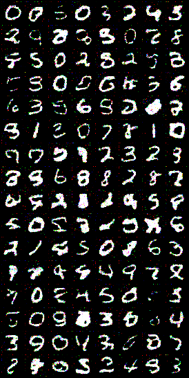
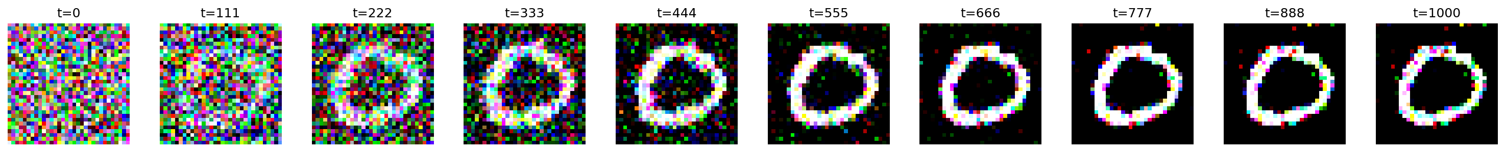
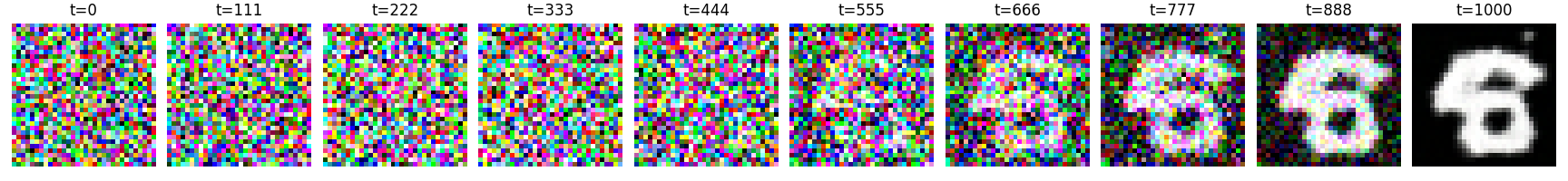
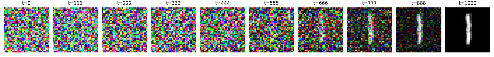
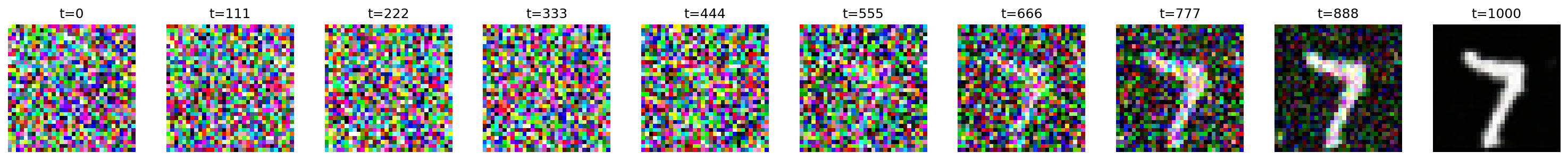
Here are some results from training on MNIST for 50 epochs, using the following configs:
BATCH_SIZE = 128
IMAGE_SIZE = 32
LR = 2e-4
NUM_TIMESTEPS = 1000
SCHEDULE_TYPE = "cosine"
SAVE_EVERY = 10
SAMPLE_EVERY = 5
Even with only ~1 hour of training on a single T4 GPU, results are pretty good:
I attempted to train on CIFAR-10 but could only get to 250 epochs due to a lack of access to GPUs, now that I’m not working in a research group anymore. Hence results are not good enough to showcase here. In the original DDPM paper, the CIFAR-10 model was trained for 800,000 iterations rather than a specific number of epochs. With a batch size of 128, this equates to approximately 2,048 epochs.
A few closing thoughts:
The math in DDPM is non-trivial to derive but everything can be simplified into a simple MSE loss, and once we have all the formulas, the implementation is surprisingly clean where each equation maps directly to a few lines of Python.
I had a lot of fun learning from and reimplementing this classic diffusion models paper - the math is actually so elegant to me!
In the next posts, I plan to discuss Improved Denoising Diffusion Probabilistic Models (Nichol & Dhariwal, 2021), which introduces the cosine schedule (already implemented here), learned variance, and other tweaks that improve sample quality significantly.
After that, we’ll get into Denoising Diffusion Implicit Models (DDIM) (Song et al., 2021), which dramatically speeds up sampling from 1000 steps to as few as 50. As you can see from the generated MNIST samples above, it took 1,000 denoising timesteps to get the final result.
Useful Resources
Theory
Code
TensorFlow:
PyTorch:
Citation
Le, Nhi. "Diffusion Models - Part 1: DDPM". halannhile.github.io (March 2026). https://halannhile.github.io/posts/ddpm/
BibTeX:
@article{nhi2025ddpm,
  title = {Diffusion Models - Part 1: DDPM},
  author = {Nhi},
  journal = {halannhile.github.io},
  year = {2026},
  month = {March},
  url = "https://halannhile.github.io/posts/ddpm/"
}