In Part 2 of the Diffusion Models series, I mentioned that Improved DDPM can match DDPM’s sample quality using only 100 steps instead of 1000, thanks to learned variance. That’s a 10x speedup and already a significant improvement. But if you’ve sat through a full 1000-step DDPM sampling loop, even 100 steps still feels slow.
Denoising Diffusion Implicit Models (DDIM; Song et al., 2021) takes a more radical approach to the speed problem. Instead of making the existing sampling loop more efficient, it asks: does the sampling loop even need to be Markovian in the first place?
The answer turns out to be no - and that single realization leads to a sampler that can generate images in as few as 10-50 steps, without any retraining. The exact same U-Net we’ve been using, trained the exact same way, just with a different sampling procedure at inference time.
The GitHub repo for my PyTorch implementation of mini-DDIM can be found here: halannhile/mini-ddim.
Table of Contents
- The bottleneck of DDPM sampling
- The key insight: training only sees marginals
- The non-Markovian forward process
- The DDIM reverse process
- Accelerated sampling
- Deterministic sampling and the latent space
Section 3: Training Optimizations
- Mixed precision (AMP)
- EMA
- Gradient accumulation
- LR warmup + cosine decay
- Gradient clipping
- Gradient checkpointing
Section 5: Recap & what’s next
Section 1: Theory
1. The bottleneck of DDPM sampling
Why is DDPM so slow to sample from? The reverse process is a Markov chain$^1$:
$$p_\theta(x_{0:T}) = p(x_T) \prod_{t=1}^{T} p_\theta(x_{t-1} | x_t)$$
$^1$What is a Markov chain?
A Markov chain is a sequence of random variables where each step only depends on the immediately preceding step, and nothing earlier. In the context of DDPM’s reverse process: to compute $x_{t-1}$, you only look at $x_t$ - not at $x_{t+1}, x_{t+2}$, etc. This “memoryless” property is what forces DDPM to take steps one at a time. You can’t skip from $x_{999}$ to $x_{500}$ directly, because the reverse transition $p_\theta(x_{500} | x_{999})$ is not defined - only single-step transitions $p_\theta(x_{t-1} | x_t)$ exist.
Each reverse step $p_\theta(x_{t-1} | x_t)$ requires one forward pass through the U-Net. Since the chain has $T=1000$ steps, generating one image takes exactly 1000 network evaluations. At inference time, this is the entire bottleneck.
One natural question is: can we just skip most of the steps? DDPM was actually tested on this, and it turns out you cannot skip arbitrarily with DDPM. Each step in the Markov chain depends on the previous one: if you skip from $t=999$ to $t=500$, the mathematical derivation of the reverse step breaks down - the transition was derived assuming you’re only moving one step at a time.
So the bottleneck isn’t just that there are 1000 steps. It’s deeper than that: the entire framework, the derivation, the math, assumes all 1000 steps happen. DDIM fixes this at the root.
2. The key insight: training only sees the marginals
When we train a DDPM, the loss we try to minimize is $L_\text{simple}$:
$$L_\text{simple} = \mathbb{E}_{t, x_0, \varepsilon} \left[ | \varepsilon - \varepsilon_\theta(\sqrt{\bar{\alpha}_t} x_0 + \sqrt{1-\bar{\alpha}_t} \varepsilon, t) |^2 \right]$$
This is just asking: given a noisy image $x_t$ at timestep $t$, predict the noise. And $x_t$ is computed using the marginal$^2$ of the forward process:
$^2$What is a marginal?
The joint distribution $q(x_1, x_2, \ldots, x_T | x_0)$ describes the distribution over every intermediate noisy image together, encoding how you step from one to the next. The marginal $q(x_t | x_0)$ is what you get when you ask: “ignoring all intermediate steps, what’s the distribution of $x_t$ given only $x_0$?” You “marginalize out” $x_1, \ldots, x_{t-1}$.
In DDPM, this marginal has a closed form: $q(x_t | x_0) = \mathcal{N}(\sqrt{\bar{\alpha}_t}, x_0,\ (1 - \bar{\alpha}_t)I)$, so you can jump directly from $x_0$ to any noisy $x_t$ in one shot without simulating the full chain. The model trained on $(x_0, x_t)$ pairs via this closed form has no idea what Markov transitions were used to get there. It only learned to denoise $x_t$ given $t$.
$$q(x_t | x_0) = \mathcal{N}(x_t; \sqrt{\bar{\alpha}_t} x_0, (1-\bar{\alpha}_t)I)$$
This marginal is fully determined by $\bar{\alpha}_t$, which comes from the noise schedule. Notice what’s not involved: the Markov transitions $q(x_t | x_{t-1})$. The training loss doesn’t care at all how you got from $x_0$ to $x_t$ along the intermediate steps - it only cares about where $x_t$ lands.
This is the key observation in the DDIM paper: the training objective constrains the marginal distributions $q(x_t | x_0)$ but says nothing about the joint distribution $q(x_{1:T} | x_0)$, i.e., the full trajectory.
In other words: many different forward processes, Markovian or not, will all produce the same marginals and therefore the same training objective. We are free to choose whatever forward process we like, as long as the marginals stay the same. The model trained under DDPM’s Markovian forward process is then valid for any of these alternative forward processes at inference time.
Formal justification (Section 3.2 of the paper)
If we write the ELBO for the non-Markovian generative process, the objective decomposes into KL terms of the form $D_\text{KL}(q_\sigma(x_{t-1} | x_t, x_0) | p_\theta(x_{t-1} | x_t))$, which depend only on the marginals $q(x_t | x_0)$, not on the specific transitions used to get there. Minimizing these terms reduces to the same $L_\text{simple}$ as DDPM for any choice of $\sigma$. See Section 3.2 of the paper Song et al., 2021 for the full derivation.
3. The non-Markovian forward process
DDIM defines a family of non-Markovian forward processes $q_\sigma$ parameterized by a vector $\sigma \in \mathbb{R}^T_{\geq 0}$. Instead of the DDPM Markov chain, it defines the reverse conditional directly:
$$q_\sigma(x_{t-1} | x_t, x_0) = \mathcal{N}\left(\sqrt{\bar{\alpha}_{t-1}} x_0 + \sqrt{1-\bar{\alpha}_{t-1} - \sigma_t^2} \cdot \frac{x_t - \sqrt{\bar{\alpha}_t} x_0}{\sqrt{1-\bar{\alpha}_t}}, \sigma_t^2 I\right)$$
This looks complex but can actually be broken down as follows:
$$\underbrace{\sqrt{\bar{\alpha}_{t-1}} x_0}_{\text{predicted clean image}} + \underbrace{\sqrt{1-\bar{\alpha}_{t-1} - \sigma_t^2} \cdot \frac{x_t - \sqrt{\bar{\alpha}_t} x_0}{\sqrt{1-\bar{\alpha}_t}}}_{\text{direction pointing toward } x_t} + \underbrace{\sigma_t \varepsilon}_{\text{noise}}$$
The mean has two components:
- A clean image direction: move toward where we predict $x_0$ to be.
- A $x_t$ direction: the residual from the current $x_t$, which points away from the clean prediction back toward the noisy image. This is what keeps the process consistent.
The $\sigma_t$ parameter controls how much stochasticity is injected at each step.
Two special cases:
- $\sigma_t = \sqrt{\frac{1-\bar{\alpha}_{t-1}}{1-\bar{\alpha}_t}} \cdot \sqrt{1 - \frac{\bar{\alpha}_t}{\bar{\alpha}_{t-1}}}$: this recovers exactly DDPM’s posterior variance $\tilde{\beta}_t$.
- $\sigma_t = 0$ for all $t$: the reverse process becomes fully deterministic. No noise is ever added. This is the DDIM case.

4. The DDIM reverse process
Since we never observe $x_0$ directly during inference, we replace it with the model’s prediction. Given a noisy image $x_t$ and the model’s predicted noise $\varepsilon_\theta(x_t, t)$, we first reconstruct a predicted clean image:
$$\hat{x}_0 = \frac{x_t - \sqrt{1-\bar{\alpha}_t} \cdot \varepsilon_\theta(x_t, t)}{\sqrt{\bar{\alpha}_t}}$$
This is the same formula I showed in Part 1 (Section 3.4), just rearranged: DDPM also computes $\hat{x}_0$ internally as an intermediate step in each denoising step. DDIM makes this the central object.
We then use $\hat{x}_0$ to compute the next state:
$$\boxed{x_{t-1} = \sqrt{\bar{\alpha}_{t-1}} \underbrace{\hat{x}_0}_{\text{predicted }x_0} + \underbrace{\sqrt{1 - \bar{\alpha}_{t-1} - \sigma_t^2} \cdot \varepsilon_\theta(x_t, t)}_{\text{direction toward }x_t} + \underbrace{\sigma_t \varepsilon}_{\text{noise}}}$$
In the deterministic case ($\sigma_t = 0$, which the paper calls DDIM):
$$x_{t-1} = \sqrt{\bar{\alpha}_{t-1}} \hat{x}_0 + \sqrt{1-\bar{\alpha}_{t-1}} \cdot \varepsilon_\theta(x_t, t)$$
Interpretation: each step is a re-noising of the predicted clean image to the correct noise level for the next step. Instead of taking a small Markov step, we try to predict the fully clean image from the current noisy one, then re-corrupt it to the right level. At $t=0$, the re-noising coefficient becomes zero and we’re left with just $\hat{x}_0$.
The $\eta$ parameter
The DDIM paper introduces a single scalar $\eta \geq 0$ that controls the amount of stochasticity:
$$\sigma_t = \eta \sqrt{\frac{1-\bar{\alpha}_{t-1}}{1-\bar{\alpha}_t}} \sqrt{1 - \frac{\bar{\alpha}_t}{\bar{\alpha}_{t-1}}}$$
- $\eta = 0$: fully deterministic (what the paper calls DDIM)
- $\eta = 1$: recovers DDPM’s posterior variance $\tilde{\beta}_t$
- $0 < \eta < 1$: a continuum between the two
This is a great design choice because it unifies DDPM and DDIM under a single framework. You can think of DDPM as DDIM with $\eta = 1$, and use $\eta$ as a dial to trade off between diversity and determinism.
5. Accelerated sampling
This is where the payoff comes. Since the non-Markovian forward process is not constrained to take one step at a time, the reverse process can skip timesteps too.
Instead of iterating over all $T=1000$ timesteps, we pick a subsequence $\tau = {\tau_1, \tau_2, \ldots, \tau_S} \subset {1, \ldots, T}$ of length $S \ll T$. The reverse process then runs over only these $S$ timesteps, jumping from $\tau_{i+1}$ to $\tau_i$ in a single step using the DDIM update.
The update formula is the same as before, just with $\bar{\alpha}_{\tau_i}$ instead of $\bar{\alpha}_{t-1}$:
$$x_{\tau_{i-1}} = \sqrt{\bar{\alpha}_{\tau_{i-1}}} \hat{x}_0 + \sqrt{1 - \bar{\alpha}_{\tau_{i-1}} - \sigma_{\tau_i}^2} \cdot \varepsilon_\theta(x_{\tau_i}, \tau_i) + \sigma_{\tau_i} \varepsilon$$
The model was still trained on all $T$ timesteps, so it can make predictions at any $\tau \in {1, \ldots, T}$. What we’ve changed is how we use those predictions at inference - instead of following every single step in the Markov chain, we take a much smaller number of larger jumps.
In practice, an evenly spaced subsequence works well: with $T=1000$ and $S=50$, you might use $\tau = {20, 40, 60, \ldots, 1000}$. The DDIM paper shows that this gives competitive sample quality compared to DDPM with 1000 steps. With $S=10$, quality degrades but is still surprisingly coherent - a generation quality level that would be completely incoherent from DDPM with the same number of steps.
6. Deterministic sampling and the latent space
The $\eta = 0$ case (fully deterministic DDIM) has a very special property that I find particularly fascinating.
Because there is zero stochasticity, the mapping from an initial noise vector $x_T$ to the final image $x_0$ is a deterministic function. The same $x_T$ always produces the same $x_0$. This means DDIM implicitly defines a bijection between the noise space $\mathcal{N}(0, I)$ and the image space - and bijections have inverses.
In practice, this means you can:
1. Encode an image into noise (DDIM inversion$^3$): run the forward DDIM process - starting from a real image $x_0$, apply the deterministic reverse formula in the forward direction to get back a noise vector $x_T$. This is exact because there’s no stochasticity to undo.
$^3$DDIM inversion
DDIM inversion is key to a whole class of editing methods. If you want to edit a real image (change “a dog sitting in a park” to “a cat sitting in a park”), you first invert the image to get its latent $x_T$, then run the forward DDIM pass conditioned on the new prompt. Because the trajectory is deterministic, the structure is preserved, i.e., you get the same pose, background, and composition, with only the specified changes applied. This is the foundation of techniques like Prompt-to-Prompt (Hertz et al., 2022) (P2P) - a technique for editing images generated by diffusion models (like Stable Diffusion) by modifying the text prompt rather than using masks or manual editing
2. Interpolate between images: take two noise vectors $x_T^{(1)}$ and $x_T^{(2)}$ (or two images inverted to their corresponding noise vectors), spherically interpolate between them, and decode each interpolated noise. Since the mapping is continuous, the decoded images smoothly transition between the two originals. This would be meaningless with DDPM since the same $x_T$ would produce a different image every time you run it. Some practical applications of interpolation are:
- If you have two real images (inverted to their noise vectors), the interpolated images between them are plausible “in-between” examples you can add to a training set,
- Or, given a generated image you like and another you like, explore the “space between them” to find intermediate variations - useful for things like face generation, product design, texture synthesis.
The practical takeaway is: DDIM (with $\eta = 0$) gives you a structured, invertible latent space essentially for free, without any changes to training. The structure comes entirely from the deterministic decoder. This is what makes DDIM so useful beyond just being faster - it’s a foundation for controllable generation and editing.
Section 2: Code
1. Overview
The codebase is a single file: ddim_single.py. As with mini-CLIP, I was inspired by Andrej Karpathy’s micro-GPT approach: everything visible in one place, no multi-module structure with complex cross-dependencies. You can edit the Config dataclass at the top instead of messing with argparse for model/diffusion settings.
There are 5 modes (I’m using CIFAR0-10 as an example here, so you’ll see this dataset name in the file paths):
Train
python ddim_single.py train
python ddim_single.py train --resume checkpoints/cifar10/ckpt_ep0100.pt
Sample - generate n images and save to samples.png
python ddim_single.py sample --checkpoint checkpoints/cifar10/latest.pt
python ddim_single.py sample --checkpoint checkpoints/cifar10/latest.pt --steps 50 --n 16 --eta 0.0
Denoise - visualize the full denoising trajectory as a grid: each row is one image going from pure noise (left) to final image (right)
python ddim_single.py denoise --checkpoint checkpoints/cifar10/latest.pt
python ddim_single.py denoise --checkpoint checkpoints/cifar10/latest.pt --steps 50 --n 4
Compare - same noise decoded at 10 / 50 / 100 / 1000 steps side-by-side
python ddim_single.py compare --checkpoint checkpoints/cifar10/latest.pt
python ddim_single.py compare --checkpoint checkpoints/cifar10/latest.pt --eta 0.0
Interpolate - slerp between two noise vectors and decode each frame
python ddim_single.py interpolate --checkpoint checkpoints/cifar10/latest.pt
python ddim_single.py interpolate --checkpoint checkpoints/cifar10/latest.pt --steps 50 --n 8 --rows 8
The default configs are for CIFAR-10 at 32×32. Switching to CelebA-HQ or LSUN at 256×256 requires changing one block at the top of the file:
cfg.dataset         = 'celeba_hq'
cfg.image_size      = 256
cfg.dim             = 128
cfg.dim_mults       = (1, 1, 2, 2, 4, 4)
cfg.batch_size      = 16
cfg.grad_accum      = 8      # effective batch = 128
cfg.grad_checkpoint = True   # needed at 256×256
cfg.checkpoint_dir  = f'./checkpoints/{cfg.dataset}'
Note: you’ll have to do some pre-work to get the CelebA-HQ and LSUN data ready before you train the model. More details on how to get these datasets are in the README.
2. The forward process
Training is identical to DDPM - same U-Net, noise schedule, and MSE loss. The DDIMScheduler precomputes $\bar{\alpha}_t$ and the training loop is unchanged:
class DDIMScheduler:
    def __init__(self):
        betas = torch.linspace(cfg.beta_start, cfg.beta_end, cfg.T, device=device)
        self.alphas_cumprod = torch.cumprod(1.0 - betas, dim=0)   # ᾱ_t, shape [T]

    def add_noise(self, x0, t, noise):
        """x_t = sqrt(ᾱ_t) x_0 + sqrt(1−ᾱ_t) ε"""
        ab = self.alphas_cumprod[t][:, None, None, None]
        return ab.sqrt() * x0 + (1 - ab).sqrt() * noise
The training forward pass (shown here without AMP (Automatic Mixed Precision in CUDA) wrapping for clarity - see Section 3 for the full optimized loop):
noise = torch.randn_like(x0)
t     = scheduler.sample_t(x0.shape[0])
x_t   = scheduler.add_noise(x0, t, noise)
pred  = model(x_t, t)
loss  = F.mse_loss(pred, noise)
The only thing that changes relative to DDPM is what we do after training, at inference time.
3. The DDIM sampler
ddim_step() implements the DDIM update equation. Given the current noisy image $x_t$, the predicted noise $\varepsilon_\theta$, and the $\eta$ parameter:
def ddim_step(self, x, t_idx, t_prev_idx, eps, eta):
    ab_t    = self.alphas_cumprod[t_idx]
    ab_prev = self.alphas_cumprod[t_prev_idx] if t_prev_idx >= 0 \
              else torch.ones(1, device=device)

    # predict clean image from current noisy image + predicted noise
    x0_pred = (x - (1 - ab_t).sqrt() * eps) / ab_t.sqrt()
    x0_pred = x0_pred.clamp(-1, 1)

    # eta=0 → deterministic (DDIM), eta=1 → stochastic (recovers DDPM)
    sigma  = eta * ((1 - ab_prev) / (1 - ab_t)).sqrt() * (1 - ab_t / ab_prev).sqrt()
    dir_xt = (1 - ab_prev - sigma ** 2).clamp(min=0).sqrt() * eps
    noise  = torch.randn_like(x) if (eta > 0 and t_prev_idx >= 0) else 0

    return ab_prev.sqrt() * x0_pred + dir_xt + sigma * noise
The sampling loop runs over a subsequence $\tau$ of $S$ evenly spaced timesteps:
@torch.no_grad()
def sample(self, model, n, steps, eta=0.0, x_start=None):
    x   = torch.randn(n, cfg.channels, cfg.image_size, cfg.image_size, device=device) \
          if x_start is None else x_start.clone()
    tau = torch.linspace(0, cfg.T - 1, steps, dtype=torch.long).flip(0).tolist()

    for i, t_idx in enumerate(tau):
        t_prev_idx = tau[i + 1] if i + 1 < len(tau) else -1
        eps        = model(x, torch.full((n,), t_idx, device=device, dtype=torch.long))
        x          = self.ddim_step(x, t_idx, t_prev_idx, eps, eta)

    return (x.clamp(-1, 1) + 1) / 2
t_prev_idx = -1 at the final step uses $\bar{\alpha}_{-1} = 1$ (the “fully clean” level), which collapses the last step to just $\hat{x}_0$ - exactly what we expect.
4. Comparing step counts
The compare mode runs the same trained model with DDIM at 10, 50, 100, and 1000 steps from the exact same noise, so the comparison is fair:
x_noise = torch.randn(n, cfg.channels, cfg.image_size, cfg.image_size, device=device)

rows = []
for steps in [*cfg.ddim_steps, cfg.T]:      # e.g. 10, 50, 100, 1000
    imgs = scheduler.sample(model, n=n, steps=steps, eta=eta, x_start=x_noise.clone())
    rows.append(imgs)

grid = make_grid(torch.cat(rows, dim=0), nrow=n, padding=2)
The result is a grid where each row is a step count (10 → 1000, top to bottom) and each column is the same image decoded at different fidelities. Passing x_start=x_noise.clone() is the key detail - content differences between columns are purely from step count, not from different starting noise.
5. Latent interpolation
The interpolate mode decodes slerp-interpolated noise vectors with $\eta = 0$:
def slerp(z0, z1, t):
    shape   = z0.shape
    z0_flat = z0.reshape(1, -1)
    z1_flat = z1.reshape(1, -1)
    norm    = z0_flat.norm()          # preserve original noise magnitude
    z0_unit = z0_flat / norm
    z1_unit = z1_flat / z1_flat.norm()
    omega   = torch.acos((z0_unit * z1_unit).sum().clamp(-1, 1))
    if omega.abs() < 1e-6:
        return ((1 - t) * z0_unit + t * z1_unit).reshape(shape) * norm
    return ((torch.sin((1-t)*omega)*z0_unit + torch.sin(t*omega)*z1_unit)
            / torch.sin(omega)).reshape(shape) * norm

z0, z1 = torch.randn(C, H, W, device=device), torch.randn(C, H, W, device=device)
noises  = torch.stack([slerp(z0, z1, t.item()) for t in torch.linspace(0, 1, n)])
imgs    = scheduler.sample(model, n=n, steps=steps, eta=0.0, x_start=noises)
eta=0.0 is required here: stochastic sampling would destroy the latent structure, giving two unrelated images at the endpoints instead of a smooth transition.
Section 3: Training Optimizations
Training diffusion models at scale requires more than just the basic loop. This section covers the optimizations I applied, ranging from ones that are relevant at any scale (EMA, LR scheduling) to ones that become necessary as image resolution increases (gradient accumulation, mixed precision, gradient checkpointing).
Optimization is an area I’ve recently dabbled in, mostly in training for now. These are my rookie early attempts, so I’m pretty sure I’ll be embarrassed looking back on them at a later time.
1. Mixed precision
Wrapping the forward pass in torch.autocast lets the model use lower-precision arithmetic where it’s safe, reducing memory and speeding up matrix multiplications:
with torch.autocast(device_type=device.type, dtype=amp_dtype, enabled=amp_dtype is not None):
    x_t  = scheduler.add_noise(x0, t, noise)
    pred = model(x_t, t)
    loss = F.mse_loss(pred, noise) / cfg.grad_accum
The dtype isn’t hardcoded - it’s selected based on the device:
def get_amp_dtype(dev):
    if not cfg.use_amp:     return None            # AMP disabled via config
    if dev.type == 'cuda':  return torch.float16   # full AMP + GradScaler
    if dev.type == 'mps':   return torch.bfloat16  # no GradScaler on MPS
    return None
On CUDA, float16 Automatic Mixed Precision (AMP) requires a GradScaler to handle loss scaling: float16 has a narrow dynamic range, so gradients can underflow to zero if they’re small. The scaler multiplies the loss by a large factor before backward, then divides the gradients back down before the optimizer step, keeping values in the representable range.
On MPS (Apple Silicon), float16 support is patchy - bfloat16 is the stable choice. Importantly, MPS doesn’t support loss scaling at all, so GradScaler is skipped entirely:
use_scaler = (amp_dtype == torch.float16)
scaler     = torch.cuda.amp.GradScaler() if use_scaler else None

# in the training loop:
if scaler:
    scaler.scale(loss).backward()
    scaler.unscale_(opt)
    nn.utils.clip_grad_norm_(model.parameters(), cfg.grad_clip)
    scaler.step(opt); scaler.update()
else:
    loss.backward()
    nn.utils.clip_grad_norm_(model.parameters(), cfg.grad_clip)
    opt.step()
2. EMA
Training weights oscillate with each stochastic gradient update. The EMA shadow copy smooths these oscillations with a running average:
class EMA:
    def __init__(self, model):
        self.shadow = deepcopy(model).eval()
        for p in self.shadow.parameters():
            p.requires_grad_(False)

    @torch.no_grad()
    def update(self, model):
        for s, m in zip(self.shadow.parameters(), model.parameters()):
            s.data.lerp_(m.data, 1 - cfg.ema_decay)   # s = decay*s + (1-decay)*m
With ema_decay=0.9999, each update moves the shadow weights 0.01% toward the current training weights - slow enough to filter out noise, fast enough to track the trend. All sampling uses ema.shadow, not model: the EMA weights consistently produce better quality images without any extra compute at inference time. This is a quality trick, not a speed trick.
3. Gradient accumulation
Diffusion models benefit from large effective batch sizes, but memory limits how much fits in one forward pass. Gradient accumulation decouples logical batch size from what fits in memory:
for step, (x0, _) in enumerate(loader):
    loss = compute_loss(x0) / cfg.grad_accum   # scale loss down
    loss.backward()                            # accumulate gradients

    if (step + 1) % cfg.grad_accum == 0:       # step every N mini-batches
        opt.step(); opt.zero_grad(); ema.update(model)
With batch_size=16 and grad_accum=8, the effective batch size is 128 - the same as CIFAR-10 in a single pass, but feasible with a 256×256 U-Net that would OOM (out-of-memory errors) at batch size 128.
Note: here’s a key detail for correctness: you need to divide the loss by cfg.grad_accum before backward. Without this, each accumulated gradient is $N\times$ larger than it should be, which effectively multiplies the learning rate by $N$.
4. LR warmup + cosine decay
def get_lr(step, total_steps):
    if step < cfg.warmup_steps:
        return cfg.lr * step / cfg.warmup_steps           # linear warmup
    progress = (step - cfg.warmup_steps) / (total_steps - cfg.warmup_steps)
    return cfg.lr * 0.5 * (1 + math.cos(math.pi * progress))  # cosine decay
The warmup prevents instability early in training when the model weights are random and gradients are large. Without it, the optimizer can take destructively large steps in the first few hundred iterations. Cosine decay smoothly reduces the learning rate as training converges, avoiding the sharp discontinuities of step decay schedules that can destabilize training near the drop points.
5. Gradient clipping
nn.utils.clip_grad_norm_(model.parameters(), cfg.grad_clip)
Diffusion models can produce large gradient spikes early in training, especially at high noise levels where the model is far from its final prediction. Clipping the gradient norm to 1.0 prevents these spikes from corrupting the weights. This runs before opt.step() every time, with or without AMP.
6. Gradient checkpointing
This optimization is only used for the 256×256 datasets (CelebA-HQ and LSUN Church). At 32×32 (CIFAR-10), the model fits comfortably in memory without it.
At 256×256, a U-Net stores activation tensors at every resolution level for the backward pass. These skip connection activations - one per encoder level, at resolutions 256, 128, 64, 32, 16, 8 - add up to the dominant memory cost at high resolution.
Gradient checkpointing$^4$ trades compute for memory: instead of storing activations, recompute them during backward when they’re needed. In ResBlock:
$^4$What is gradient checkpointing?
During the forward pass, PyTorch stores all intermediate activations (outputs of each layer) so they’re available for computing gradients during the backward pass. At high resolution, these stored tensors consume a large chunk of GPU memory.
Gradient checkpointing discards those activations after the forward pass and recomputes them on-the-fly during backward when they’re actually needed. You pay with extra compute but recover significant memory, which lets you train with larger batch sizes or higher resolutions that would otherwise OOM.
def forward(self, x, t):
    if self._ckpt and self.training:
        return grad_ckpt(self._fwd, x, t, use_reentrant=False)
    return self._fwd(x, t)
I apply it selectively to the deeper half of the encoder (i >= n_levels // 2), not the whole network. This is the best memory/recompute tradeoff for a diffusion U-Net:
- Shallow blocks (high resolution, fewer channels) have larger activations by total element count - a 256×256 block with 128 channels is ~8M elements vs. ~32K for an 8×8 block with 512 channels. So checkpointing them would save more raw memory, but recomputing large convolutions over full-resolution spatial maps is expensive and slows training noticeably.
- Deep blocks (low resolution, many channels) are cheap to recompute - small spatial maps mean the extra backward pass is fast. They also avoid complications with skip connections, which pass tensors from encoder to decoder and need to remain available during the backward pass.
Here’s my recommendation: you can start with deep-half checkpointing. If you’re still hitting OOM, extend it progressively toward shallower levels until it fits.
Section 4: Results
I trained on CIFAR-10 for 400 epochs. Ideally, it could be more, around 800 epochs.
The CIFAR-10 dataset has 10 classes: ‘airplane’, ‘automobile’, ‘bird’, ‘cat’, ‘deer’, ‘dog’, ‘frog’, ‘horse’, ‘ship’, ‘truck’, of size 3x32x32, i.e. 3-channel color images of 32x32 pixels in size.
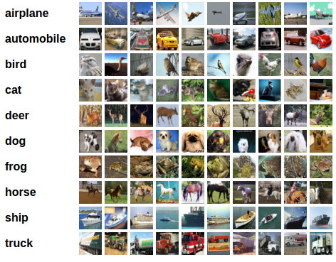
(Image source: PyTorch)
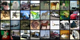
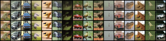
The compare mode (same noise → DDIM at 10/50/100/1000 steps) shows clearly that 50 steps produces images visually indistinguishable from 1000 steps. Even the 10-step samples are recognizably similar in content to their 1000-step counterparts - you can see the same object and rough structure, just with less texture detail.
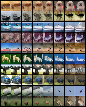
The interpolate mode shows smooth, continuous transitions in image space - exactly what you’d expect from a model that has learned a meaningful latent space.
Section 5: Recap & what’s next
DDIM is one of those papers where the key insight is almost obvious in hindsight, but wasn’t obvious at the time. The observation that $L_\text{simple}$ only depends on marginals had been sitting in the DDPM derivation the whole time - DDIM just noticed it and took it seriously.
What I find compelling about DDIM is that it’s not just a speed trick. The deterministic sampler and the structured latent space are genuinely new capabilities that you get for free once you abandon the Markovian constraint. DDIM inversion (encoding a real image back to noise) is fundamental to a whole generation of editing and control methods that I’ll cover later in this series.
For the next post, I’m planning to go into Score-Based Generative Models (Song & Ermon, 2019/2020), which provides the continuous-time perspective on diffusion. It’s a very different mathematical framing that ultimately connects to DDPM and DDIM, but through stochastic differential equations.
Useful Resources
1. Theory
DDIM paper: Denoising Diffusion Implicit Models - Song et al., 2021.
Lil’Log - What are diffusion models? - still the best single reference; Section 4 covers DDIM specifically.
→ I actually just realized Professor Huang has a list of key Diffusion Models papers categorized very neatly into Training, Guidance, Resolution & Speed, which you might find helpful in compartmentalizing your understanding of the space, though they’re not ordered chronologically:
Training
- Sohl-Dickstein et al. 2015 - Deep Unsupervised Learning using Nonequilibrium Thermodynamics
- Ho et al. 2020 - Denoising Diffusion Probabilistic Models
- Luo 2022 - Understanding Diffusion Models: A Unified Perspective
- Karras et al. 2022 - Elucidating the Design Space of Diffusion-Based Generative Models
- Karras et al. 2023 - Analyzing and Improving the Training Dynamics of Diffusion Models
Guidance
- Dhariwal and Nichol 2021 - Diffusion Models Beat GANs on Image Synthesis
- Ho and Salimans 2022 - Classifier-Free Diffusion Guidance
- Sander Dieleman 2022 - Guidance: a cheat code for diffusion models
- Sander Dieleman 2023 - The geometry of diffusion guidance
Resolution
- Ho et al. 2021 - Cascaded Diffusion Models for High Fidelity Image Generation
- Saharia et al. 2022 - Photorealistic Text-to-Image Diffusion Models with Deep Language Understanding
- Rombach et al. 2021 - High-Resolution Image Synthesis with Latent Diffusion Models
- Vahdat et al. 2021 - Score-based Generative Modeling in Latent Space
- Podell et al. 2023 - SDXL: Improving Latent Diffusion Models for High-resolution Image Synthesis
- Hoogeboom et al. 2023 - Simple diffusion: End-to-end diffusion for high resolution images
- Chen et al. 2023 - On the importance of noise scheduling for diffusion models
- Gu et al. 2023 - Matryoshka Diffusion Models
Speed
- (we are here) Song et al. 2021 - Denoising Diffusion Implicit Models
- Salimans and Ho 2022 - Progressive Distillation for Fast Sampling of Diffusion Models
- Meng et al. 2023 - On Distillation of Guided Diffusion Models
- Song et al. 2023 - Consistency Models
- Luo et al. 2023 - Latent Consistency Models: Synthesizing High-Resolution Images with Few-Step Inference
- Luo et al. 2023 - LCM-LoRA: A Universal Stable-Diffusion Acceleration Module
- Sauer et al. 2023 - Adversarial Diffusion Distillation
- Yin et al. 2023 - One-step Diffusion with Distribution Matching Distillation
2. Code
- ermongroup/ddim - the official PyTorch implementation from the authors.
Citation
Le, Nhi. "Diffusion Models - Part 3: DDIM". halannhile.github.io (April 2026). https://halannhile.github.io/posts/ddim/
BibTeX:
@article{nhi2026ddim,
  title = {Diffusion Models - Part 3: DDIM},
  author = {Nhi},
  journal = {halannhile.github.io},
  year = {2026},
  month = {April},
  url = "https://halannhile.github.io/posts/ddim/"
}