Multimodal AI has always been an area I am personally very fascinated by, because I believe our understanding of the world comes from more than just language - it’s also vision and audio (and touch and smell, of course, but that might be outside the scope of what I’m capable of exploring in my own time). Since working at Adobe, I’ve grown an even deeper appreciation for how hard it is to teach machines to reason about the visual world, and beyond that, the physical world.
There’s a reason the saying goes “an image is worth a thousand words” - a single photo carries information about lighting, mood, texture, depth, object relationships, and implied story that would take paragraphs to describe in language. For humans, all of that arrives instantly. For machines, that richness is exactly the problem: none of it is written down, structured, or can be learned from text alone.
This is the problem that CLIP (Contrastive Language–Image Pre-Training; Radford et al., 2021) takes a serious first step toward solving. CLIP was the paper that made vision-language models (VLMs) mainstream. Take Stable Diffusion, DALL·E, or any image search system in the last few years, CLIP - or something inspired by it - is almost certainly involved somewhere.
One of the earliest and most fundamental questions I had regarding multimodal AI was: “how does a model learn that this image and this sentence are about the same thing?”. Nobody explicitly labels every image-text pair as “matching” or “not matching”. Yet CLIP can take a photo of a golden retriever and rank “a dog playing in the grass” above “a cat sitting on a couch” with remarkable accuracy.
The GitHub repo for my PyTorch implementation of mini-CLIP can be found here: halannhile/mini-clip.
Table of Contents
- The problem CLIP solves
- The core idea: a shared embedding space
- The two encoders
- Contrastive learning and the InfoNCE loss
- Training at scale
- Zero-shot transfer
- A few caveats
- Dataset
- Image encoder
- Text encoder
- The similarity matrix and InfoNCE loss
- Temperature
- Optimizer and learning rate
- MPS optimizations
- Retrieval evaluation
Section 3: Results from the trained model
Section 4: Recap & what’s next
Section 1: Theory
1. The problem CLIP solves
Before CLIP, training a vision model that understood images in terms of language was expensive and not very scalable. The standard approach was supervised learning on fixed label sets: e.g., take ImageNet’s 1,000 categories, collect millions of labeled images, train a classifer. It works - but only for those 1,000 categories. If you want to recognize something new, you’ll need new labeled data, a new output head, and another training run.
The deeper problem I see is that the world doesn’t come pre-labeled. Photos on the internet come with captions, alt text, surrounding context - in other words, unstructured language, not structured labels. This free-form supervision signal is vastly richer than any human-curated dataset can be.
The key insight from CLIP is: instead of predicting labels, predict which caption belongs to which image, which looks something like this: given millions of image-text pairs scraped from the internet, the model learns that the photo of the Golden Gate Bridge and “San Francisco’s most iconic architecture” go together, while that same photo and “a cat on a sofa” do not.
As simple as this reframing sounds, turns out it unlocked a very different kind of generalization. I will explain why in the rest of this blog.
2. The core idea: a shared embedding space
This is a high-dimensional vector space that both images and text get projected into. The goal is to learn projections $f$ and $g$ such that:
$$\text{similarity}(f(\text{image}),\ g(\text{caption})) \text{ is high if they match, low otherwise}$$
where “similarity” is measured by the cosine similarity$^1$ between two vectors:
$^1$Quick recap on cosine similarity
Cosine similarity measures the angle between two vectors, not their distance. Two vectors pointing in exactly the same direction have cosine similarity 1.0; perpendicular vectors have 0.0; opposite vectors have -1.0. Crucially, it ignores the magnitude of the vectors - only direction matters. This is exactly the property we want: a short caption and a long caption describing the same image should both point in the same direction in embedding space, even if their raw vector lengths differ.
What we want to get is a space where semantically related things cluster together, regardless of whether they’re images or text. So it could be that a photo of Eiffel Tower and Statue of Liberty end up near each other, although no explicit visual similarity was ever taught.
In other words, the model has no explicit notion of “dog” as a category. It has learned that certain visual patterns and certain word patterns tend to co-occur, and compressed that co-occurrence into geometric proximity. The structure emerges from the training signal, not from any hard-coded concept of what a “dog” is.
3. The two encoders
CLIP has two separate neural networks - one for images, one for text - each independently mapping their input into the shared embedding space.
3.1. The image encoder
The image encoder $f(\cdot)$ maps an image to a fixed-size embedding vector. The CLIP paper experiments with two architectures:
- ResNet variants (ResNet-50, ResNet-101, and scaled-up versions up to ResNet-50x64)
- Vision Transformer (ViT) variants (ViT-B/32$^2$, ViT-B/16, ViT-L/14)
$^2$What does ViT-B/32 mean?
The notation breaks down as: architecture size / patch size. B = Base (86M parameters), L = Large (307M parameters). The number after the slash is the patch size in pixels - so ViT-B/32 splits the input image into 32×32 pixel patches, while ViT-B/16 uses 16×16 patches. Smaller patches = more tokens = finer detail = higher compute cost. ViT-L/14 (Large, 14×14 patches) is the most expensive variant and the one that performs best in CLIP.
Both work, but ViT-L/14 performs best at scale. I’ll go much deeper into ViT in Post 2 of the series - it’s a fascinating architecture and deserves its own post. For now, the key thing is that both encoders produce a single vector $\mathbf{v}_i \in \mathbb{R}^d$ for each image $i$.
Before being used for similarity computation, this vector is L2-normalized (projected onto the unit hypersphere):
$$\hat{\mathbf{v}}_i = \frac{\mathbf{v}_i}{|\mathbf{v}_i|}$$
After L2 normalization, cosine similarity reduces to a dot product: $\text{sim}(\hat{\mathbf{u}}, \hat{\mathbf{v}}) = \hat{\mathbf{u}} \cdot \hat{\mathbf{v}}$. It means we never need to compute vector norms during training (they’re all 1.0 by construction) and the optimization landscape is cleaner.
3.2. The text encoder
The text encoder $g(\cdot)$ maps a text string to a vector in the same $d$-dimensional space. It’s a Transformer (Vaswani et al., 2017) - specifically, a 63M-parameter model with 12 layers, 512-wide, and 8 attention heads - essentially a GPT-2-scale model.
The input text is tokenized using a byte-pair encoding (BPE)$^3$ vocabulary of 49,408 tokens.
$^3$What is BPE tokenization?
BPE is a compression algorithm adapted for text. It starts with individual characters, then iteratively merges the most frequent adjacent pair into a new token - repeating until a fixed vocabulary size is reached. The result is a vocabulary of common subwords: frequent words like “the” get their own token, while rarer words get split into meaningful pieces (“unbelievable” → “un”, “believ”, “able”). BPE handles out-of-vocabulary words very well since any word can be decomposed into known subword tokens.
The sequence is bracketed with [SOS] (start of sequence) and [EOS] (end of sequence) tokens. The representation at the [EOS] position$^4$ is used as the text embedding - a single vector for the entire sequence.
$^4$Why use the [EOS] token’s representation and not, say, an average of all tokens?
In a causal (GPT-style) transformer, each token can only attend to previous tokens. This means the [EOS] token is the only position that has “seen” every token in the sequence - it accumulates information from all preceding tokens through the attention mechanism. Averaging all token representations would mix early tokens (which haven’t seen the full sequence) with later ones, diluting the global context. The [EOS] representation is the cleanest single-vector summary of the full sequence.
Note: BERT-style encoders use a [CLS] token at the start for the same reason, but via bidirectional attention.
The text vector is then also L2-normalized, same as the image embeddings.
Important note: the two encoders (text- and image-encoders) have separate weights, and are trained jointly from scratch. What does this mean? There’s no weight sharing between the image and text branches. They only interact through the contrastive loss, i.e., the sole signal pushing the two spaces together is the training objective itself. I find this to be a really interesting and elegant approach: there’s no complicated cross-modal fusion happening here, just two encoders and a loss that forces them to agree with each other.
3.3. Linear projection heads
I’ll keep this part brief since it’s a small design choice. Each encoder outputs an embedding in its own internal dimensionality (e.g. 768 for ViT-B/32, 512 for the text transformer). These get projected into the shared embedding dimension $d$ via learned linear projections - simple weight matrices with no bias and no activation function:
$$\hat{\mathbf{v}}_i = \text{L2Norm}(W_I \cdot \text{ImageEncoder}(x_i))$$ $$\hat{\mathbf{u}}_i = \text{L2Norm}(W_T \cdot \text{TextEncoder}(t_i))$$
Note that there are no non-linearities in the projection heads - the encoders learn rich representations in their own space, and the linear projections align those spaces without distorting them.
4. Contrastive learning and the InfoNCE loss
This is the part that made everything click for me, so I want to spend more time here.
The training objective of CLIP is simple: maximize the cosine similarity between matched image-text pairs, and minimize it between mismatched pairs.. The following sections will explain how to turn this goal into a loss function that works at scale.
4.1. The setup: a matrix of similarities
Take a minibatch of $N$ image-text pairs: ${(x_1, t_1), (x_2, t_2), …, (x_N, t_N)}$, where $(x_i, t_i)$ is a matched pair (an image and its caption scraped together from the web).
CLIP computes embeddings for all $N$ images and all $N$ texts:
$$\mathbf{I} = [\hat{\mathbf{v}}_1, \hat{\mathbf{v}}_2, …, \hat{\mathbf{v}}_N] \in \mathbb{R}^{N \times d}$$ $$\mathbf{T} = [\hat{\mathbf{u}}_1, \hat{\mathbf{u}}_2, …, \hat{\mathbf{u}}_N] \in \mathbb{R}^{N \times d}$$
Then computes an $N \times N$ matrix of pairwise cosine similarities:
$$S_{ij} = \hat{\mathbf{v}}_i \cdot \hat{\mathbf{u}}_j$$
$S_{ij}$ is the similarity between image $i$ and text $j$. The diagonal entries $S_{ii}$ are matched pairs. The off-diagonal entries $S_{ij}$ (where $i \neq j$) are mismatched - image $i$ with some other image’s caption.
The goal: make the diagonal entries large, and the off-diagonal ones small.
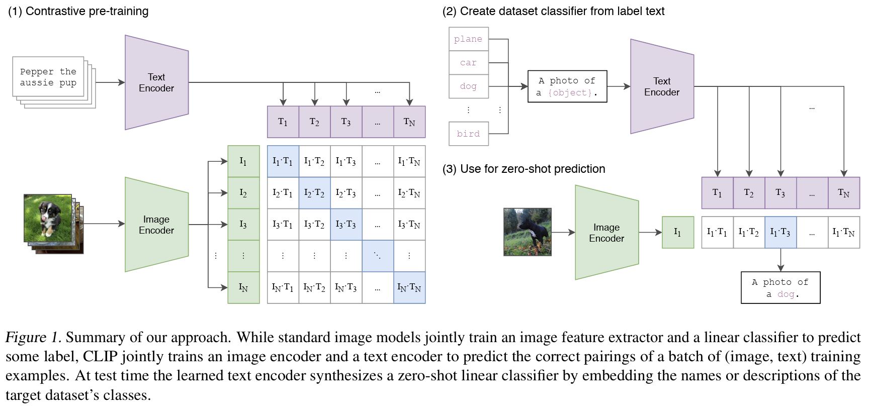
4.2. Why the N×N setup is so powerful
Look at that matrix again. For a minibatch of $N$ image-text pairs, CLIP computes $N \times N = N^2$ similarities in one shot. Only $N$ of those are correct matches (the diagonal). The remaining $(N^2 - N)$ are all mismatched pairs - and the model has to learn to score them lower than the correct match.
That means each minibatch of $N$ pairs gives CLIP $N$ positive examples and $(N^2 - N)$ negative examples for free.
With $N = 32{,}768$ (the batch size CLIP uses), that’s roughly 1 billion negative pairs per step. The model has to distinguish the correct caption from 32,767 competing captions for every single image, and vice versa.
Compare that to supervised classification, where a model just distinguishes between 1,000 fixed categories. In CLIP’s setup, every minibatch is a fresh set of ~1 billion unique discrimination problems. The representations have to be genuinely good to survive that.
This is what the loss function of CLIP needs to operationalize: for each image, rank all $N$ texts by similarity and push the correct one to the top - and do the same in the other direction.
4.3. The InfoNCE loss
CLIP does the task of maximizing diagonal entries with a symmetric cross-entropy loss, also known as the InfoNCE loss$^5$ (van den Oord et al., 2018).
$^5$What is InfoNCE loss?
Information Noise Contrastive Estimation. The “Info” part refers to mutual information: maximizing InfoNCE is equivalent to maximizing a lower bound on the mutual information between the two views (image and text). The “NCE” part refers to “noise contrastive estimation”, an older technique for training unnormalized probabilistic models by distinguishing real data from synthetic noise samples. Basically, InfoNCE is a contrastive loss: for each image, the model should give a high score to its matching caption and low scores to all other captions in the batch (and vice versa). In CLIP, those wrong image-text matches act as the “noise” negatives, and it pushes true pairs closer, while mismatched pairs apart.
For each image $i$, treat row $S_{i, \cdot}$ as a classification problem over $N$ classes, where the “correct” class is index $i$ (the matched text). The loss is a cross-entropy over softmaxed similarities:
$$\mathcal{L}_{\text{img} \rightarrow \text{txt}} = -\frac{1}{N} \sum_{i=1}^{N} \log \frac{\exp(S_{ii} / \tau)}{\sum_{j=1}^{N} \exp(S_{ij} / \tau)}$$
In simple terms: for each image, rank all $N$ texts by similarity, and push the correct one to the top.
Symmetrically, for each text $j$, treat column $S_{\cdot, j}$ as a classification problem over $N$ classes where the correct class is index $j$:
$$\mathcal{L}_{\text{txt} \rightarrow \text{img}} = -\frac{1}{N} \sum_{j=1}^{N} \log \frac{\exp(S_{jj} / \tau)}{\sum_{i=1}^{N} \exp(S_{ij} / \tau)}$$
The final loss is the average of both:
$$\boxed{\mathcal{L}_{\text{CLIP}} = \frac{1}{2} \left( \mathcal{L}_{\text{img} \rightarrow \text{txt}} + \mathcal{L}_{\text{txt} \rightarrow \text{img}} \right)}$$
4.4. The temperature parameter $\tau$
$\tau$ is a learnable temperature$^6$ parameter - initialized to $\tau = 0.07$ and optimized jointly with the encoder weights (clipped to a maximum of 100 to prevent training instability).
$^6$What does temperature control (in AI models)?
Broadly, temperature controls how sharp vs. flat a probability distribution is.
- Lower temperature → sharper distribution: the model becomes more confident and deterministic. In generative models, this usually means less diversity, more repetitive/“safe” outputs, and fewer surprising samples.
- Higher temperature → flatter distribution: probabilities spread out more, so outputs become more diverse/random. This increases variety and creativity, but also raises the chance of incoherent or lower-quality outputs.
A useful rule of thumb in generation: low temperature for reliability/consistency, high temperature for exploration/diversity.
In CLIP specifically, temperature rescales similarities before softmax, controlling how strongly the model separates matched pairs from mismatched pairs.
Low $\tau$: the softmax puts almost all probability mass on the highest similarity entry. The loss becomes very unforgiving - even a slightly lower similarity to the correct pair gets penalized harshly.
High $\tau$: the distribution flattens out, all entries look similar, and the loss gradient weakens.
Making $\tau$ learnable rather than fixed is a small but important choice - the right temperature turns out to be data-dependent, so letting the model figure it out during training works better than setting it manually.
5. Training at scale
The scale of CLIP’s training is not incidental but is actually the whole point.
CLIP was trained on WIT (WebImageText), a dataset of 400 million image-text pairs collected from the web - this is OpenAI’s internal dataset and was never released to the public. The open-source community released alternatives: LAION-400M and later LAION-5B (5.85 billion image-text pairs) are the most widely used. If you train an open-source CLIP model today - via the open_clip library - you’re almost certainly training on a LAION subset.
Note: LAION-5B has known issues with noisy and mismatched captions, which is one reason finetuning on a clean domain-specific dataset can so dramatically improve performance on that domain. I’ll write a dedicated blog post on finetuning later.
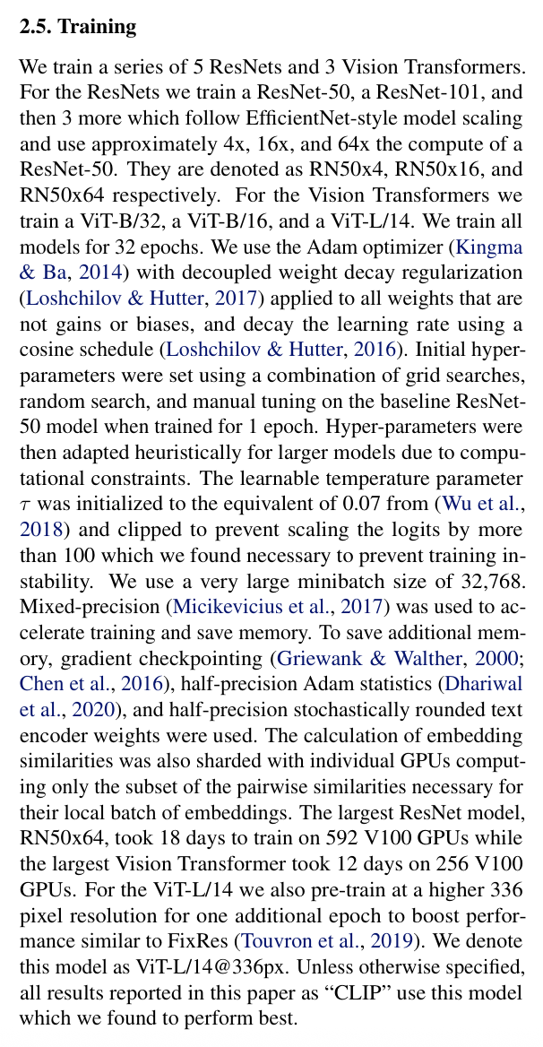
As you can see from the image above, the scale at which CLIP was trained is massive.
Why does scale matter so much in the case of CLIP training?
A large minibatch size of 32,768 means more negative pairs per step. So a representation that correctly ranks the right caption to an image, above 32,767 alternatives, must have internalized genuinely discriminative features. In other words, more negatives = harder task = better representations.
Remember that the whole WiT dataset came from web-scale supervision, not human annotation. 400M captions from the internet describe concepts that no curated label set could ever do. The model has to develop representations across an enormous range of visual concepts, and not limited by the categories defined by a dataset curator. This leads to diversity in the concept space of the trained CLIP model.
Both of these points, as a result of the massive training scale, is the core reason CLIP generalizes so broadly. This would have been practically impossible before large-scale distributed training became accessible. So even though the idea of contrastive learning goes back years, CLIP is the product of when we finally have the compute to take it seriously.
For a view into how contrastive learning builds up to CLIP, I recommend Andrej Karpathy’s lecture on Transformers for the architectural building blocks, and Lil’Log’s post on contrastive representation learning for the learning framework. I’d also read SimCLR: A Simple Framework for Contrastive Learning of Visual Representations (Chen et al., 2020) before reading CLIP and it made the contrastive objective much clearer.
Another interesting point worth mentioning: CLIP tested multiple image backbones: ResNet and Vision Transformer (ViT), and they found that: ViT scaled better and achieved stronger performance at large sizes.
6. Zero-shot transfer
Reference: Section 3.1. Zero-Shot Transfer of the CLIP paper.
A nice reward for all of this is zero-shot transfer - the ability to do classification tasks the model was never explicitly trained on, without any fine-tuning. This is what I was most impressed about after reading the paper.
The way it works is, say you want CLIP to classify images into $K$ categories ${c_1, c_2, …, c_K}$. Instead of training a linear probe on top of the image encoder, you:
- Construct $K$ text prompts, one per class:
"a photo of a {class}". - Encode each prompt with the text encoder to get $K$ text embeddings.
- Encode the new image with the image encoder.
- Predict the class whose text embedding has the highest cosine similarity to the image embedding.
No labeled examples needed in this whole process. On ImageNet, CLIP’s zero-shot accuracy matches a fully supervised ResNet-50 trained on 1.28 million labeled images. On several specialized datasets - Stanford Cars, Food-101, EuroSAT - it actually outperforms supervised models trained specifically on those datasets.
7. A few caveats
7.1. Prompt matters
There was one finding from the paper that I didn’t expect: the exact phrasing of text prompts significantly affects performance. "a photo of a {class}" consistently beats the bare class name "{class}". For fine-grained categories, domain-specific templates help even more: "a satellite photo of {class}" for EuroSAT, "a photo of the {class}, a type of food" for Food-101.
My first reaction was that this felt fragile and a bit unsatisfying. But it actually makes sense once you think about how the model was trained: it learned associations between full phrases and visual patterns, not just isolated words. “Satellite” activates different visual features than “photo” because it appeared in different contexts in the training data. The model picked that up.
7.2. Limitation of zero-shot CLIP
Zero-shot CLIP has a well-known failure mode: fine-grained visual distinctions within a narrow domain.
On CUB-200 (200 bird species), CLIP’s zero-shot accuracy is around 57%, below supervised models trained specifically on birds. On MNIST, it only reaches ~76%, well below a simple supervised CNN. The reason is the same in both cases: CLIP has seen birds and handwritten digits on the internet, but its representations were never forced to discriminate at the granularity these benchmarks require.
This is exactly why finetuning CLIP matters so much in practice. A generic CLIP embedding of “a photo of a Patagonia jacket” won’t necessarily be amazing at distinguishing between Patagonia’s different product lines. A CLIP finetuned on Patagonia’s actual product catalog will.
Section 2: Code
You can find my PyTorch implementation of mini-clip here.
My implementation is a single-file PyTorch mini-CLIP (clip_single.py), trained on Flickr30k (~29.8k images, 5 captions each). I was definitely inspired by Andrej Karpathy’s microgpt to create a reimplementation with no abstractions, no package structure, everything visible in one file.
I mean, isn’t this beautiful:
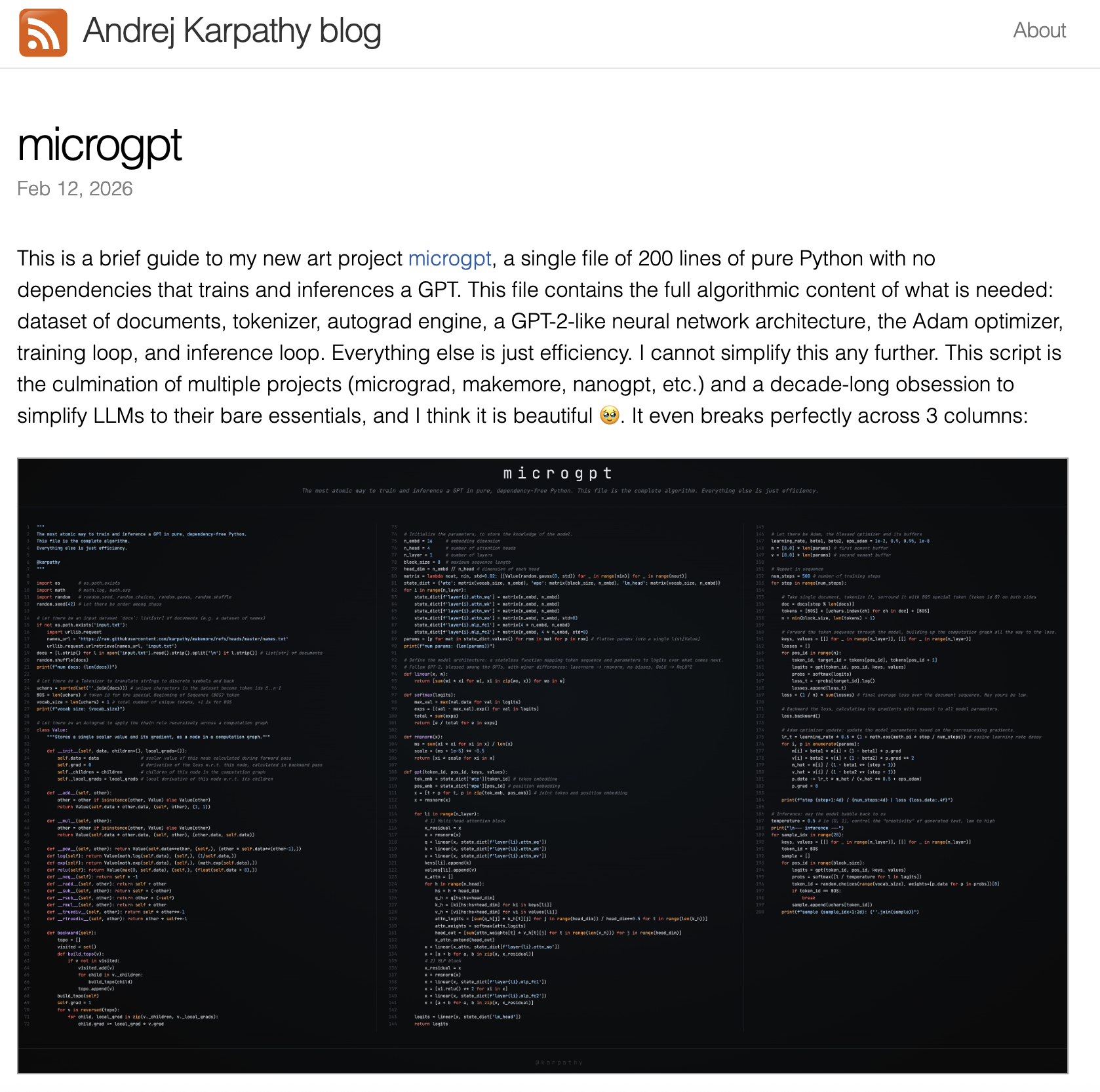
There are 2 main reasons I will take this approach moving forward. One, it challenged me to figure out what the absolute core essentials of the model are. Second, it significantly speeds up my coding time, which then allows me to read and reimplement more papers (TL;DR: I realized I spent way too much time on DDPM and Improved DDPM, which clearly isn’t sustainable).
1. Dataset
Flickr30k is small by CLIP standards, but it uses a standard benchmark partition called the Karpathy split (~29.8k train / 1k val / 1k test), so retrieval results are directly comparable to other papers. The HuggingFace version stores all ~31k rows in a single table - I filter by a split column to get the actual train/val/test buckets.
Each image has 5 human-written captions. During training, I randomly pick one of the 5 per step so the model sees varied descriptions across epochs. During val and retrieval eval, I use fixed caption indices for reproducibility.
def __getitem__(self, idx):
    img_idx, cap_idx = self.samples[idx]
    row     = self.data[img_idx]
    image   = self.transform(row["image"].convert("RGB"))
    # during training pick a random caption; during val use a fixed one
    caption = random.choice(row["caption"]) if self.is_train \
              else row["caption"][cap_idx]
    # tokenize returns shape [1, L], take [0] to get [L]
    tokens  = openai_clip.tokenize([caption], context_length=cfg.context_length,
                                    truncate=True)[0]
    return image, tokens
2. Image encoder
Training a ViT from scratch on only 29k images doesn’t really work - there’s just not enough data for the model to learn good visual features. So instead I use a pretrained vit_base_patch32_224 from timm, which already understands visual concepts from ImageNet. The idea is to finetune it to align with the text embeddings, rather than learn vision from scratch.
timm.create_model(..., num_classes=0) removes the classification head and returns the raw CLS token vector (768-dim for ViT-Base), which I then project down to the shared 256-dim embedding space with a linear layer.
One thing to be careful about here: the pretrained ViT was trained with ImageNet normalization (mean=[0.485, 0.456, 0.406], std=[0.229, 0.224, 0.225]), not the CLIP-specific constants sometimes seen in other implementations. Using the wrong normalization would feed off-distribution pixels to the pretrained backbone.
# standard ImageNet normalization - the pretrained ViT was trained on these,
# so we use them instead of the CLIP-specific constants
CLIP_MEAN = [0.485, 0.456, 0.406]
CLIP_STD  = [0.229, 0.224, 0.225]

class VisionEncoder(nn.Module):
    """pretrained ViT backbone (timm) + linear projection to shared embed_dim."""
    def __init__(self):
        super().__init__()
        # num_classes=0 removes the classifier head - backbone returns the CLS vector directly
        self.backbone = timm.create_model(
            cfg.vit_model,
            pretrained=True,
            num_classes=0,
        )
        vit_out_dim = self.backbone.num_features   # 768 for vit_base
        # projection head: dropout → linear; dropout regularizes the small dataset overfitting
        self.proj = nn.Sequential(
            nn.Dropout(p=0.1),
            nn.Linear(vit_out_dim, cfg.embed_dim, bias=False),
        )
        nn.init.trunc_normal_(self.proj[1].weight, std=0.02)

    def forward(self, x):
        x = self.backbone(x)   # [B, 768]
        return F.normalize(self.proj(x), dim=-1)
3. Text encoder
The text encoder is a small causal transformer trained from scratch: 6 layers, 512-wide, 8 attention heads - roughly GPT-2 small scale. I use OpenAI’s BPE tokenizer (via the clip package) with a 49,408-token vocabulary and a max sequence length of 77.
The sequence is summarized by the hidden state at the [EOS] position - in CLIP’s tokenization, this is always the highest token id in the row. Since the transformer is causal, [EOS] is the only position that has seen the full sequence, so it’s the cleanest single-vector summary of the whole caption.
def forward(self, tokens):
    B, N = tokens.shape
    # token embedding + positional embedding - same idea as GPT
    x = self.tok_emb(tokens) + self.pos_emb[:N]
    x = self.ln(self.blocks(x))
    # the EOS token has the highest id in the sequence - use its position as the summary
    eos = tokens.argmax(dim=-1)
    return F.normalize(self.proj(x[torch.arange(B), eos]), dim=-1)
4. The similarity matrix and InfoNCE loss
For a batch of $N$ image-text pairs, I compute all $N \times N$ cosine similarities in one matrix multiply (both embeddings are L2-normalized, so dot product = cosine similarity). The diagonal entries are matched pairs; everything off-diagonal is a negative. Then I apply symmetric cross-entropy: each image tries to identify its matched caption among all $N$ texts, and vice versa.
img = self.encode_image(images)   # [B, D], unit vectors
txt = self.encode_text(tokens)    # [B, D], unit vectors

# dot product = cosine sim (vectors are already unit norm)
# diagonal of the [B, B] matrix are the matched image-caption pairs
logits  = img @ txt.T * scale
# label for sample i is i - i.e. the correct match is always on the diagonal
labels  = torch.arange(len(img), device=img.device)

# two cross-entropies: one treating images as queries, one treating captions
loss = (F.cross_entropy(logits, labels) +
        F.cross_entropy(logits.T, labels)) / 2
5. Temperature
The temperature $\tau$ is a learnable parameter initialized to 0.07 (same as the original CLIP paper). I store it as log_tau and clamp it so $\tau$ stays in $[0.01, 100]$ - this prevents the loss from blowing up or collapsing early in training. scale = exp(log_tau) is 1/τ, which multiplies the logits before softmax.
# log(1/0.07) ≈ 2.659 → τ starts at 0.07 (same default as openai's CLIP)
self.log_tau = nn.Parameter(torch.tensor(2.659))

# clamp so τ stays in [0.01, 100] - avoids loss blowing up or collapsing
log_tau = self.log_tau.clamp(math.log(1/100), math.log(1/0.01))
scale   = log_tau.exp()   # this is 1/τ
6. Optimizer and learning rate
I use AdamW with weight decay 0.2, but exclude weight decay from biases, LayerNorm parameters, embeddings, and log_tau - decaying those would wrongly pull scale/shift parameters toward zero.
Since the ViT backbone is pretrained, I give it a much lower learning rate (100x lower than the projection heads and text encoder). The backbone’s features are already good, so I don’t want aggressive updates to undo that. I also freeze the backbone for the first 2 epochs so the projection heads can stabilize before the backbone starts moving - without this, the pretrained features shift too fast and the model starts overfitting quickly on the small dataset.
(Lots of training time was wasted until I could figure out why the model was overfitting).
The lr schedule is a linear warmup over 2 epochs, then cosine decay to 0. Each param group has its initial_lr stamped at the start so the schedule applies as a multiplier, which preserves the backbone/other lr ratio throughout training.
backbone_lr = cfg.lr * cfg.backbone_lr_scale
return torch.optim.AdamW(
    [{"params": backbone_decay,   "weight_decay": cfg.weight_decay, "lr": backbone_lr},
     {"params": backbone_nodecay, "weight_decay": 0.0,              "lr": backbone_lr},
     {"params": other_decay,      "weight_decay": cfg.weight_decay, "lr": cfg.lr},
     {"params": other_nodecay,    "weight_decay": 0.0,              "lr": cfg.lr}],
    lr=cfg.lr, betas=(0.9, 0.98), eps=1e-6,
)

# freeze backbone at the start so the projection heads can warm up first
if cfg.freeze_backbone_epochs > 0:
    for p in model.image_encoder.backbone.parameters():
        p.requires_grad = False

# unfreeze backbone once we're past the freeze period
if epoch == cfg.freeze_backbone_epochs + 1:
    for p in model.image_encoder.backbone.parameters():
        p.requires_grad = True
7. MPS optimizations
Since I’m training on a Mac with Apple Silicon, there are a few things worth calling out that are specific to MPS.
bfloat16 autocast. I use torch.autocast with dtype=torch.bfloat16 during the forward pass. This reduces memory usage and speeds up matrix multiplications on the MPS backend. I picked bfloat16 over float16 specifically because bfloat16 has the same dynamic range as float32 (just less precision), so gradients don’t underflow - which is a real problem with float16 on small models. GradScaler (the usual fix for float16 underflow) isn’t well supported on MPS anyway, so bfloat16 is the cleaner choice here.
# bfloat16 autocast on MPS - reduces memory and speeds up compute
# GradScaler is not supported on MPS, but bfloat16 has a wider dynamic range
# than float16 so gradient underflow isn't a problem
if cfg.use_amp and device.type == "mps":
    _amp_ctx = torch.autocast(device.type, dtype=torch.bfloat16)
pin_memory=False. MPS uses unified memory (CPU and GPU share the same physical memory), so pinning tensors for faster CPU→GPU transfer doesn’t apply and actually triggers a warning. I disable it explicitly.
persistent_workers=True. DataLoader workers are kept alive between batches rather than being respawned each epoch. This saves a noticeable amount of overhead when loading Flickr30k images.
set_to_none=True in zero_grad. Instead of filling gradients with zeros, PyTorch deallocates the gradient tensors entirely. This is slightly faster and uses less memory since the tensors don’t exist until the next backward pass.
optimizer.zero_grad(set_to_none=True) # slightly faster than filling with 0
CPU thread configuration. Since MPS offloads compute to the GPU but data preprocessing still runs on CPU, tuning cpu_num_threads and cpu_num_interop_threads matters. The defaults in Config are set to work well for Apple Silicon, but you can adjust them if you notice CPU becoming a bottleneck during data loading.
I hope this section gives you some insights on how you can speed up training on Mac with Apple Sillicon if that’s also the deep learning machine you can afford currently. Obviously, it’s still painfully slow, but I just observe for a few epochs that things are going well, leave them running and go on a hike and hope that nothing breaks in the meantime.
8. Retrieval evaluation
The standard Flickr30k retrieval benchmark has two directions:
- Image→Text (I→T): for each of the 1,000 test images, rank all 5,000 captions by cosine similarity and check if any of the image’s 5 ground-truth captions appear in the top-K.
- Text→Image (T→I): for each of the 5,000 captions, rank all 1,000 images and check if the parent image is in the top-K.
I report R@1, R@5, and R@10 for both directions. R@1 is the strictest - the correct match has to be ranked first.
# image → text: the 5 correct captions for image i are at indices [5i, 5i+5)
i2t = recall_at_k(sim,   lambda i: set(range(5*i, 5*i+5)))
# text → image: caption j belongs to image j // 5
t2i = recall_at_k(sim.T, lambda j: {j // 5})

print("\nFlickr30k retrieval:")
print(f"  I→T  R@1: {i2t['R@1']:.1f}%  R@5: {i2t['R@5']:.1f}%  R@10: {i2t['R@10']:.1f}%")
print(f"  T→I  R@1: {t2i['R@1']:.1f}%  R@5: {t2i['R@5']:.1f}%  R@10: {t2i['R@10']:.1f}%")
For example, this is the result at epoch 10:
1000 images, 5000 captions

Flickr30k retrieval:
  I→T  R@1: 50.3%  R@5: 80.0%  R@10: 87.9%
  T→I  R@1: 37.0%  R@5: 67.2%  R@10: 76.5%
18:46:58 |   New best R@1 avg: 43.6% → saved best.pt
Section 3: Results from the trained model
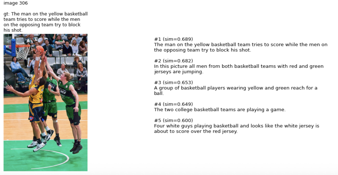
Visualizing the image, the ground truth caption, and the top 5 retrieved captions:
Here are some examples where the top 1 retrieved caption matches with the ground truth caption. You can see that the top 2-5 retrieved captions are also close matches with ground truth:
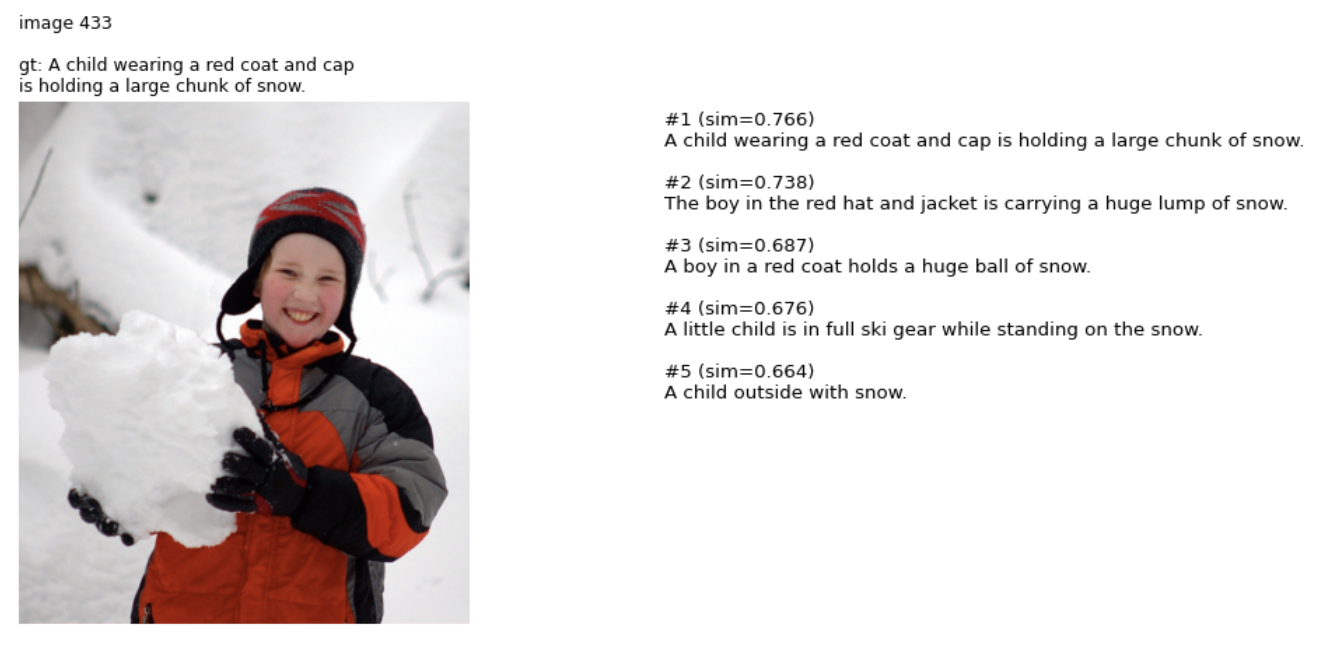
Top 1 retrieved caption matches with ground truth
Top 1 retrieved caption matches with ground truth
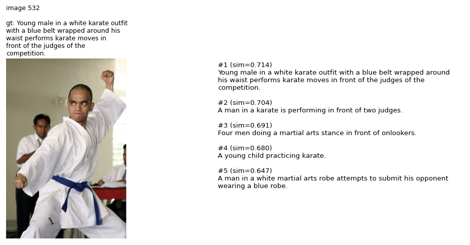
Top 1 retrieved caption matches with ground truth
And here are some examples where the top 1 retrieved caption does not match with the ground truth caption, but the ground truth caption is still in the list of top 5 retrieved captions. The top 1 is actually a really good match with ground truth, just not exactly correct. Same as above, all retrieved captions are really good descriptions of the image:
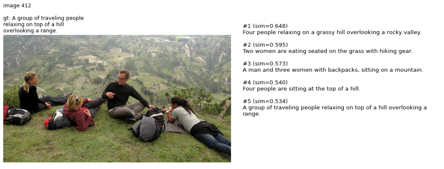
Ground truth caption is among the top 5 retrieved captions
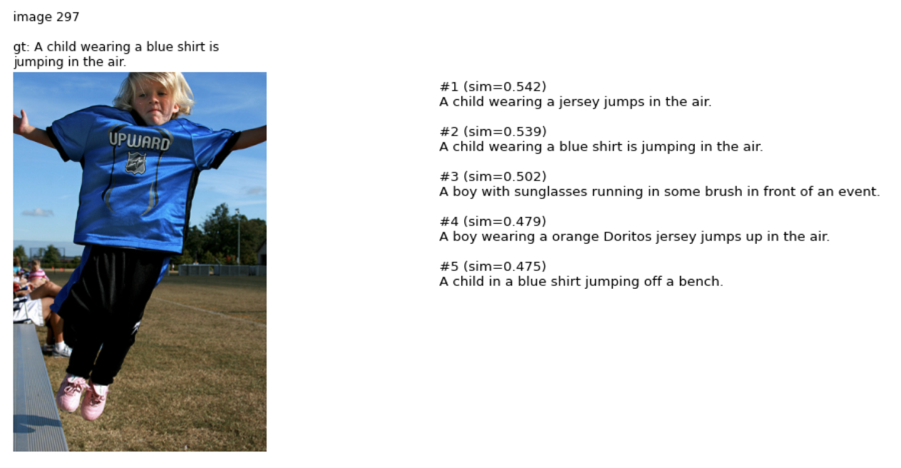
Ground truth caption is among the top 5 retrieved captions
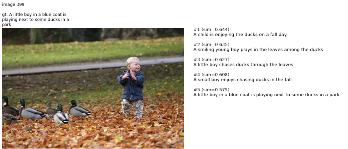
Ground truth caption is among the top 5 retrieved captions
Section 4: Recap & what’s next
CLIP is no longer the absolute peak of vision-language research, and not always SOTA (e.g. research has moved toward coupling stronger text decoders with vision encoders (like BLIP-2) for better performance; newer Generative Multimodal Large Language Models (MLLMs) perform better at complex visual reasoning or understanding spatial relationships).
But I still want to start this series with CLIP because it remains a staple in production AI for its efficiency and strong foundational capabilities. A few enterprise use cases where CLIP still plays an important role (at least from what I observe at Adobe) are: image search, brand alignment scoring, conditional generation, and custom model finetuning:
Image search: Embed your entire asset library with the image encoder. At query time, embed the search query with the text encoder. Retrieve by cosine similarity.
Brand alignment: Embed a set of brand-approved images. For any generated image, compute its cosine similarity to that brand cluster. Higher similarity = more on-brand.
Conditional generation: The text encoder from CLIP is used directly in Stable Diffusion and many other diffusion models to convert a text prompt into the conditioning vector that guides image generation.
Custom model finetuning: Textual inversion literally optimizes a new token embedding in CLIP’s text encoder space to represent a new concept. DreamBooth: Fine Tuning Text-to-Image Diffusion Models for Subject-Driven Generation (Ruiz et al., 2022) updates the model’s weights to learn a new subject, but it still leans on the pretrained semantic knowledge - usually coming from a CLIP-style text encoder - to keep the concept grounded.
This may seem a little backwards, but in the next post, I’ll go deep on the Vision Transformer (ViT) paper: An Image is Worth 16x16 Words: Transformers for Image Recognition at Scale (Google Research, 2021) - the architecture behind CLIP’s most powerful image models and one that has since become the default backbone for many modern vision and multimodal systems. Understanding ViT well will be very useful when you go through the rest of this series.
Useful resources
Official CLIP resources
CLIP: Learning Transferable Visual Models From Natural Language Supervision - Radford et al., 2021. Section 2 (approach) and Section 3.1 (zero-shot transfer) are useful reads.
Papers
Representation Learning with Contrastive Predictive Coding - van den Oord et al., 2018. The original InfoNCE paper. Section 2.2 derives the loss.
A Simple Framework for Contrastive Learning of Visual Representations (SimCLR) - Chen et al., 2020. I’d read this before CLIP, it made the contrastive objective much clearer in the simpler vision-only setting.
Blog posts
- Lil’Log - Contrastive Representation Learning - imo the best single resource for understanding the family of contrastive objectives that CLIP belongs to. Read through SimCLR and MoCo before getting to CLIP.
Code
mlfoundations/open_clip - an open-source reproduction of CLIP with support for many architectures and datasets. It is widely used in research and production, and many recent papers rely on it when they refer to using CLIP because: 1. original CLIP training code from OpenAI was not fully released, 2. OpenCLIP provides scalable training infrastructure, 3. OpenCLIP supports many pretrained checkpoints.
Citation
Le, Nhi. "Multimodal AI - Part 1: CLIP". halannhile.github.io (April 2026). https://halannhile.github.io/posts/clip/
BibTeX:
@article{nhi2026clip,
  title = {Multimodal AI - Part 1: CLIP},
  author = {Nhi},
  journal = {halannhile.github.io},
  year = {2026},
  month = {April},
  url = "https://halannhile.github.io/posts/clip/"
}